1.3 Path integral quantization of a Bose particle

The canonical quantization of a classical system has been discussed in the previous section. There the main role was played by the Hamiltonian and the Lagrangian did not show up at all. In the present section, it will be shown that there exists a quantization process, called the path integral quantization, based heavily on the Lagrangian.

1.3.1 Path integral quantization

We start our analysis with one-dimensional systems. Let $\hat{x}(t)$ be the position operator in the Heisenberg picture. Suppose the particle is found at $x_i$ at time $t_i(>0)$ . Then the probability amplitude of finding this particle at $x_f$ at later time $t_f(>t_i)$ is

$$⟨x_f,t_f|x_i,t_i⟩\text{\hspace{1em}(1.79)}$$

where the vectors are defined in the Heisenberg picture, 12

$$\hat{x}\left(t_i\right)|x_i,t_i⟩=x_i|x_i,t_i⟩\text{\hspace{1em}(1.80)}$$

$$\hat{x}\left(t_f\right)|x_f,t_f⟩=x_f|x_f,t_f⟩.\text{\hspace{1em}(1.81)}$$

The probability amplitude (1.79) is also called the transition amplitude.

Let us rewrite the probability amplitude in terms of the Schrödinger picture. Let $\hat{x}=\hat{x}(0)$ be the position operator with the eigenvector

$$\hat{x}|x⟩=x|x⟩.\text{\hspace{1em}(1.82)}$$

Since $\hat{x}$ has no time dependence, its eigenvector should be also time independent. If

$$\hat{x}\left(t_i\right)={\mathrm{e}}^{\mathrm{i}\hat{H}{t}_i}\hat{x}{\mathrm{e}}^{-\mathrm{i}\hat{H}{t}_i}\text{\hspace{1em}(1.83)}$$

is substituted into (1.80), we obtain

$${\mathrm{e}}^{\mathrm{i}\hat{H}{t}_i}\hat{x}{\mathrm{e}}^{-\mathrm{i}\hat{H}{t}_i}|x_i,t_i⟩=x_i|x_i,t_i⟩.$$

By multiplying ${\mathrm{e}}^{-\mathrm{i}\hat{H}{t}_i}$ from the left, we find

$$\hat{x}[{\mathrm{e}}^{-\mathrm{i}\hat{H}{t}_i}|x_i,t_i⟩]=x_i[{\mathrm{e}}^{-\mathrm{i}\hat{H}{t}_i}|x_i,t_i⟩].$$

This shows that the two eigenvectors are related as

$$|x_i,t_i⟩={\mathrm{e}}^{\mathrm{i}\hat{H}{t}_i}|x_i⟩.\text{\hspace{1em}(1.84)}$$

Similarly, we have

$$|x_f,t_f⟩={\mathrm{e}}^{\mathrm{i}\hat{H}{t}_f}|x_f⟩,\text{\hspace{1em}(1.85)}$$

from which we obtain

$$⟨x_f,t_f|=⟨x_f|{\mathrm{e}}^{-\mathrm{i}\hat{H}{t}_f}.\text{\hspace{1em}(1.86)}$$

From these results, we express the probability amplitude in the Schrödinger picture as

$$⟨x_f,t_f|x_i,t_i⟩=⟨x_f|e^{-\mathrm{i}\hat{H}(t_f-t_i)}|x_i⟩.\text{\hspace{1em}(1.87)}$$

In general, the function

$$h(x,y;\beta )\equiv ⟨x|e^{-\hat{H}\beta }|y⟩\text{\hspace{1em}(1.88)}$$

is called the heat kernel of $\hat{H}$ . This nomenclature originates from the similarity between the Schrödinger equation and the heat equation. The amplitude (1.87) is the heat kernel of $\hat{H}$ with imaginary $\beta$ :

$$⟨x_f,t_f|x_i,t_i⟩=h\left(x_f,x_i;\mathrm{i}\left(t_f-t_i\right)\right).\text{\hspace{1em}(1.89)}$$

Now the amplitude (1.87) is expressed in the path integral formalism. To this end, we consider the case in which $t_f-t_i=\epsilon$ is an infinitesimal positive number. Let us put $x_i=x$ and $x_f=y$ to simplify the notation and suppose the Hamiltonian is of the form

$$\hat{H}=\frac{{\hat{p}}^2}{2m}+V(\hat{x}).\text{\hspace{1em}(1.90)}$$

We first prove the following lemma.

Lemma 1.2

Let $a$ be a positive constant. Then

$${\int }_{-\infty }^{\infty }{\mathrm{e}}^{-\mathrm{i}a{p}^2}\mathrm{d}p=\sqrt{\frac{\pi }{\mathrm{i}a}}.\text{\hspace{1em}(1.91)}$$

Proof

The integral is different from an ordinary Gaussian integral in that the coefficient of $p^2$ is a pure imaginary number. First replace $p$ by $z=x+\mathrm{i}y$ . The integrand $\exp (-\mathrm{i}a{z}^2)$ is analytic in the whole $z$ -plane. Now change the integration contour from the real axis to the one shown in figure 1.1. Along path 1, we have $\mathrm{d}z=\mathrm{d}x$ and hence this path gives the same contribution as the original integration (1.91). The contribution from paths 2 and 4 vanishes as $R\to \infty$ . Noting that the variable along path 3 is $z=(1-\mathrm{i})x$ , we evaluate the contribution from this path as

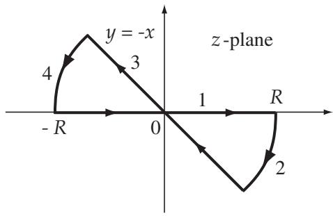
Figure 1.1. The integration contour.

$$(1-\mathrm{i}){\int }_{\infty }^{-\infty }{\mathrm{e}}^{-2a{x}^2}\mathrm{d}x=-{\mathrm{e}}^{-\mathrm{i}\pi /4}\sqrt{\frac{\pi }{a}}.$$

The summation of all the contribution must vanish due to Cauchy’s theorem and, hence,

$${\int }_{-\infty }^{\infty }\mathrm{d}p{\mathrm{e}}^{-\mathrm{i}a{p}^2}={\mathrm{e}}^{-\mathrm{i}\pi /4}\sqrt{\frac{\pi }{a}}=\sqrt{\frac{\pi }{\mathrm{i}a}}.$$

Now this lemma is employed to obtain the heat kernel for an infinitesimal time interval.

Proposition 1.2

Let $\hat{H}$ be a Hamiltonian of the form (1.90) and $\epsilon$ be an infinitesimal positive number. Then for any $x,y\in \mathbb{R}$ , we find that

$$\begin{array}{rl}⟨x|{\mathrm{e}}^{-\mathrm{i}\hat{H}\epsilon }|y⟩& =\frac{1}{\sqrt{2\pi \mathrm{i}\epsilon }}\exp [\mathrm{i}\epsilon \{\frac{m}{2}{\left(\frac{(x-y{)}^2}{\epsilon }\right)}^2\\ & -V\left(\frac{x+y}{2}\right)\}+\mathcal{O}\left({\epsilon }^2\right)+\mathcal{O}\left(\epsilon (x-y{)}^2\right)].\end{array}\text{\hspace{1em}(1.92)}$$

Proof

The completeness relation for the momentum eigenvectors is inserted into the LHS of (1.92) to yield

$$\begin{array}{rl}⟨x|{\mathrm{e}}^{-\mathrm{i}\hat{H}\epsilon }|y⟩& =\int \mathrm{d}k⟨x|{\mathrm{e}}^{-\mathrm{i}\epsilon \hat{H}}|k⟩⟨k|y⟩\\ & =\int \frac{\mathrm{d}k}{2\pi }{\mathrm{e}}^{-\mathrm{i}ky}{\mathrm{e}}^{-i\epsilon {\hat{H}}_x}{\mathrm{e}}^{\mathrm{i}kx}\end{array}$$

where

$${\hat{H}}_x=-\frac{1}{2m}\frac{{\mathrm{d}}^2}{\mathrm{d}{x}^2}+V(x).$$

Now we find from the commutation relation of ${\partial }_x\equiv \mathrm{d}/\mathrm{d}x$ and ${\mathrm{e}}^{\mathrm{i}kx}$ that

$${\partial }_x{\mathrm{e}}^{\mathrm{i}kx}=\mathrm{i}k{\mathrm{e}}^{\mathrm{i}kx}+{\mathrm{e}}^{\mathrm{i}kx}{\partial }_x={\mathrm{e}}^{\mathrm{i}kx}(\mathrm{i}k+{\partial }_x).$$

Repeated application of this commutation relation yields

$${\partial }_x^n{\mathrm{e}}^{\mathrm{i}kx}={\mathrm{e}}^{\mathrm{i}kx}(\mathrm{i}k+{\partial }_x{)}^n(n=0,1,2,\dots )$$

from which we obtain

$${\mathrm{e}}^{-\mathrm{i}\epsilon \left[-{\partial }_x^2/2m+V(x)\right]}{\mathrm{e}}^{\mathrm{i}kx}={\mathrm{e}}^{\mathrm{i}kx}{\mathrm{e}}^{-\mathrm{i}\epsilon \left[-(\mathrm{i}k+{\partial }_x{)}^2/2m+V(x)\right]}.$$

Therefore,

$$\begin{array}{rl}⟨x|{\mathrm{e}}^{-\mathrm{i}\hat{H}\epsilon }|y⟩& =\int \frac{\mathrm{d}k}{2\pi }{\mathrm{e}}^{\mathrm{i}k(x-y)}{\mathrm{e}}^{-\mathrm{i}\epsilon [-(\mathrm{i}k+{\partial }_x{)}^2/2m+V(x)]}\\ & =\int \frac{\mathrm{d}k}{2\pi }{\mathrm{e}}^{-\mathrm{i}[\epsilon k^2/2m-k(x-y)]}{\mathrm{e}}^{-\mathrm{i}\epsilon [-\mathrm{i}k{\partial }_x/m-{\partial }_x^2/2m+V(x)]}\cdot 1\end{array}$$

where the ‘1’ at the end of the last line is written explicitly to remind us of the fact ${\partial }_{x}1=0$ . If we further put $p=\sqrt{\epsilon /2m}k$ and expands the last exponential function in the last line, we obtain

$$\begin{array}{rl}& ⟨x|{\mathrm{e}}^{-\mathrm{i}\epsilon \hat{H}}|y⟩=\sqrt{\frac{2m}{\epsilon }}{\mathrm{e}}^{\mathrm{i}m(x-y{)}^2/2\epsilon }\int \frac{\mathrm{d}p}{2\pi }{\mathrm{e}}^{-\mathrm{i}[p+\sqrt{m/2\epsilon }(x-y){]}^2}\\ & \times \sum _{n=0}^{\infty }\frac{(-\mathrm{i}\epsilon {)}^n}{n!}{\left[\mathrm{i}\sqrt{\frac{2}{\epsilon m}}p{\partial }_x-\frac{{\partial }_x^2}{2m}+V(x)\right]}^n\cdot 1.\end{array}$$

If we put $q=p+\sqrt{m/2\epsilon }(x-y)$ and use lemma 1.2, we obtain:

$$\begin{array}{rl}& ⟨x|{\mathrm{e}}^{-\mathrm{i}\epsilon \hat{H}}|y⟩=\sqrt{\frac{2m}{\epsilon }}{\mathrm{e}}^{\mathrm{i}m(x-y{)}^2/2\epsilon }\int \frac{\mathrm{d}q}{2\pi }{\mathrm{e}}^{-\mathrm{i}{q}^2}\\ & \times [1+(-\mathrm{i}\epsilon )V(x)+\frac{(-{\epsilon }^2)}{2}\frac{(-\mathrm{i})}{\epsilon }(x-y){\partial }_{x}V(x)\\ & +\mathcal{O}\left({\epsilon }^2\right)+\mathcal{O}\left(\epsilon |x-y{|}^2\right)]\\ & =\sqrt{\frac{m}{2\pi \mathrm{i}\epsilon }}{\mathrm{e}}^{\mathrm{i}\epsilon (m/2)[(x-y)/\epsilon {]}^2}\\ & \times \exp \left[-\mathrm{i}\epsilon V\left(\frac{x+y}{2}\right)+\mathcal{O}({\epsilon }^2)+\mathcal{O}(\epsilon |x-y{|}^2)\right].\end{array}$$

Thus, the proposition has been proved.

$\square$

Note that the average value $(x+y)/2$ appeared as the variable of $V$ in (1.92). This prescription is often called the Weyl ordering.

It is found from (1.92) that the integrand oscillates very rapidly for $|x-y|>\sqrt{\epsilon }$ and it can be regarded as zero in the sense of distribution (the Riemann-Lebesgue theorem). Therefore, as $x-y<\epsilon$ , the exponent of (1.92) approaches the action for an infinitesimal time interval $[0,\epsilon ]$ ,

$$\Delta S={\int }_0^{\epsilon }\mathrm{d}t\left[\frac{m}{2}{v}^2-V(x)\right]\simeq \left[\frac{m}{2}{v}^2-V(x)\right]\epsilon \text{\hspace{1em}(1.93)}$$

where $v=(x-y)/\epsilon$ is the average velocity and $x$ is the average position.

Equation (1.92) also satisfies the boundary condition for $\epsilon \to 0$

$$⟨x\mid {\mathrm{e}}^{-\mathrm{i}{\hat{H}}_{\epsilon }}|y⟩\stackrel{\epsilon \to 0}{\to }⟨x|y⟩=\delta (x-y).\text{\hspace{1em}(1.94)}$$

This can be shown by noting that

$${\int }_{-\infty }^{\infty }dx\sqrt{\frac{m}{2\pi \mathrm{i}\epsilon }}{e}^{\mathrm{i}m(x-y{)}^2/2\epsilon }=1.$$

The transition amplitude (1.79) for a finite time interval is obtained by infinitely repeating the transition amplitude for an infinitesimal time interval one after another. Let us first divide the interval $t_f-t_i$ into $n$ equal intervals,

$$\epsilon =\frac{t_f-t_i}{n}.$$

Put $t_0=t_i$ and $t_k=t_0+\epsilon k$ ( $0\le k\le n$ ). Clearly $t_n=t_f$ . Insert the completeness relation

$$1=\int \mathrm{d}{x}_k|x_k,t_k⟩⟨x_k,t_k|(1\le k\le n-1)$$

for each instant of time $t_k$ into (1.79) to yield

$$\begin{array}{rl}& ⟨x_f,t_f|x_i,t_i⟩=⟨x_f,t_f|\int \mathrm{d}{x}_{n-1}|x_{n-1},t_{n-1}⟩⟨x_{n-1},t_{n-1}|\\ & \times \int \mathrm{d}{x}_{n-2}|x_{n-2},t_{n-2}⟩\cdots \int \mathrm{d}{x}_1|x_1,t_1⟩⟨x_1,t_1\mid x_0,t_0⟩.\end{array}$$

Let us consider here the limit $\epsilon \to 0$ , namely $n\to \infty$ . Proposition 1.2 states that for an infinitesimal $\epsilon$ , we have

$$⟨x_k,t_k|x_{k-1},t_{k-1}⟩\simeq \sqrt{\frac{m}{2\pi \mathrm{i}\epsilon }}{\mathrm{e}}^{\mathrm{i}\Delta S_k}$$

where

$$\Delta S_k=\epsilon \left[\frac{m}{2}{\left(\frac{x_k-x_{k-1}}{\epsilon }\right)}^2-V\left(\frac{x_{k-1}+x_k}{2}\right)\right].$$

Therefore, we find

$$⟨x_f,t_f\mid x_i,t_i⟩=\underset{n\to \infty }{\lim }{\left(\frac{m}{2\pi \mathrm{i}\epsilon }\right)}^{n/2}\int \prod _{j=1}^{n-1}\mathrm{d}{x}_j\exp \left(\mathrm{i}\sum _{k=1}^n\Delta S_k\right).\text{\hspace{1em}(1.95)}$$

If $n-1$ points $x_1,x_2,\dots ,x_{n-1}$ are fixed, we obtain a piecewise linear path from $x_0$ to $x_n$ via these points. Then we define $S(\{x_k\})={\sum }_k\Delta S_k$ , which in the limit $n\to \infty$ can be written as

$$S\left(\left\{x_k\right\}\right)\stackrel{n\to \infty }{⟶}S[x(t)]={\int }_{t_i}^{t_f}\mathrm{d}t\left[\frac{m}{2}{v}^2-V(x)\right].\text{\hspace{1em}(1.96)}$$

Note, however, that the $S[x(t)]$ defined here is formal; the variables $x_k$ and $x_{k-1}$ need not be close to each other and hence $v=(x_k-x_{k-1})/\epsilon$ may diverge. This transition amplitude is written symbolically as

$$\begin{array}{rl}⟨x_f,t_f|x_i,t_i⟩& =\int \mathcal{D}x\exp \left[\mathrm{i}{\int }_{t_i}^{t_f}\mathrm{d}t\left(\frac{m}{2}{v}^2-V(x)\right)\right]\\ & =\int \mathcal{D}x\exp \left[i{\int }_{t_i}^{t_f}\mathrm{d}tL(x,\dot{x})\right]\end{array}\text{\hspace{1em}(1.97)}$$

which is called the path integral representation of the transition amplitude. It should be stressed again that the $v$ is not well defined and that this expression is just a symbolic representation of the limit (1.95).

The integration measure is understood as

$$\int \mathcal{D}x=\text{s u m m a t i o n o v e r a l l p a t h s}x(t)\text{w i t h}x\left(t_i\right)=x_i,x\left(t_f\right)=x_f\text{\hspace{1em}(1.98)}$$

see figure 1.2. Although $\mathcal{D}x$ or $S(\{x_k\})$ is ill defined in the limit $n\to \infty$ , the amplitude $⟨x_f,t_f|x_i,t_i⟩$ constructed from $\mathcal{D}x$ and $S(\{x_k\})$ together is well defined and hence meaningful. This point is clarified in the following example.

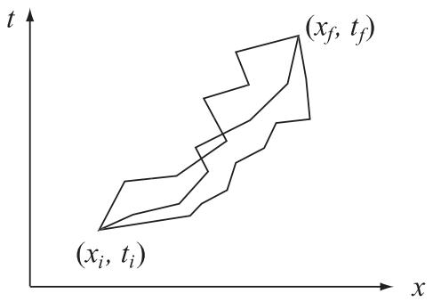
Figure 1.2. All the paths with fixed endpoints are considered in the path integral. The integrand $\exp [\mathrm{i}S(\{x_k\})]$ is integrated over these paths.

Example 1.5

Let us work out the transition amplitude of a free particle moving on the real axis with the Lagrangian

$$L=\frac{1}{2}m{\dot{x}}^2.\text{\hspace{1em}(1.99)}$$

The canonical conjugate momentum is $p=\partial L/\partial \dot{x}=m\dot{x}$ and the Hamiltonian is

$$H=p\dot{x}-L=\frac{p^2}{2m}.\text{\hspace{1em}(1.100)}$$

The transition amplitude is calculated within the canonical quantum theory as

$$\begin{array}{rl}⟨x_f,t_f|x_i,t_i⟩& =⟨x_f|{\mathrm{e}}^{-\mathrm{i}\hat{H}T}|x_i⟩=\int \mathrm{d}p⟨x_f|{\mathrm{e}}^{-\mathrm{i}\hat{H}T}|p⟩⟨p|x_i⟩\\ & =\int \frac{\mathrm{d}p}{2\pi }{\mathrm{e}}^{\mathrm{i}p\left(x_f-x_i\right)}{\mathrm{e}}^{-\mathrm{i}T\left(p^2/2m\right)}\\ & =\sqrt{\frac{m}{2\pi \mathrm{i}T}}\exp \left(\frac{\mathrm{i}m{\left(x_f-x_i\right)}^2}{2T}\right)\end{array}\text{\hspace{1em}(1.101)}$$

where $T=t_f-t_i$ .

This result is obtained using the path integral formalism next. The amplitude is expressed as

$$\begin{array}{rl}& ⟨x_f,t_f|x_i,t_i⟩=\underset{n\to \infty }{\lim }{\left(\frac{m}{2\pi \mathrm{i}\epsilon }\right)}^{n/2}\int \mathrm{d}{x}_1\dots \mathrm{d}{x}_{n-1}\\ & \exp \left[\mathrm{i}\epsilon \sum _{k=1}^n\frac{m}{2}{\left(\frac{x_k-x_{k-1}}{\epsilon }\right)}^2\right]\end{array}\text{\hspace{1em}(1.102)}$$

where $\epsilon =T/n$ . After scaling the coordinates as

$$y_k={\left(\frac{m}{2\epsilon }\right)}^{1/2}{x}_k$$

the amplitude becomes

$$\begin{array}{rl}& ⟨x_f,t_f|x_i,t_i⟩=\underset{n\to \infty }{\lim }{\left(\frac{m}{2\pi \mathrm{i}\epsilon }\right)}^{n/2}{\left(\frac{2\epsilon }{m}\right)}^{(n-1)/2}\\ & \int \mathrm{d}{y}_1\dots \mathrm{d}{y}_{n-1}\exp \left[\mathrm{i}\sum _{k=1}^n{\left(y_k-y_{k-1}\right)}^2\right].\end{array}\text{\hspace{1em}(1.103)}$$

It can be shown by induction (exercise) that

$$\int \mathrm{d}{y}_1\dots \mathrm{d}{y}_{n-1}\exp \left[\mathrm{i}\sum _{k=1}^n(y_k-y_{k-1}{)}^2\right]={\left[\frac{(\mathrm{i}\pi {)}^{(n-1)}}{n}\right]}^{1/2}{\mathrm{e}}^{\mathrm{i}(y_n-y_0{)}^2/n}.$$

Taking the limit $n\to \infty$ , we finally obtain

$$\begin{array}{rl}⟨x_f,t_f|x_i,t_i⟩& =\underset{n\to \infty }{\lim }{\left(\frac{m}{2\pi \mathrm{i}\epsilon }\right)}^{n/2}{\left(\frac{2\pi \mathrm{i}\epsilon }{m}\right)}^{(n-1)/2}\frac{1}{\sqrt{n}}{\mathrm{e}}^{\mathrm{i}m(x_f-x_i{)}^2/(2n\epsilon )}\\ & =\sqrt{\frac{m}{2\pi \mathrm{i}T}}\exp \left[\frac{\mathrm{i}m{\left(x_f-x_i\right)}^2}{2T}\right].\end{array}\text{\hspace{1em}(1.104)}$$

It should be noted here that the exponent is the classical action. In fact, if we note that the average velocity is $v=(x_f-x_i)/(t_f-t_i)$ , the classical action is found to be

$$S_{\mathrm{cl}}={\int }_{t_i}^{t_f}\mathrm{d}t\frac{1}{2}m{v}^2=\frac{m(x_f-x_i{)}^2}{2(t_f-t_i)}.$$

It happens in many exactly solvable systems that the transition amplitude takes the form

$$⟨x_f,t_f|x_i,t_i⟩=A{\mathrm{e}}^{\mathrm{i}{S}_{\mathrm{cl}}},\text{\hspace{1em}(1.105)}$$

where all the effects of quantum fluctuation are taken into account in the prefactor $A$ .

1.3.2 Imaginary time and partition function

Suppose the spectrum of a Hamiltonian $\hat{H}$ is bounded from below. Then it is always possible, by adding a positive constant to the Hamiltonian, to make $\hat{H}$ positive definite;

$$\mathrm{Spec}\hat{H}=\left\{0<E_0\le E_1\le E_2\le \dots \right\}.\text{\hspace{1em}(1.106)}$$

It has been assumed for simplicity that the ground state is not degenerate. The spectral decomposition of ${\mathrm{e}}^{-\mathrm{i}\hat{H}t}$ given by

$${\mathrm{e}}^{-\mathrm{i}\hat{H}t}=\sum _n{\mathrm{e}}^{-\mathrm{i}{E}_{n}t}|n⟩⟨n|\text{\hspace{1em}(1.107)}$$

is analytic in the lower half-plane of $t$ , where $\hat{H}|n⟩=E_n|n⟩$ . Introduce the Wick rotation by the replacement

$$t=-\mathrm{i}\tau (\tau \in {\mathbb{R}}_{+})\text{\hspace{1em}(1.108)}$$

where ${\mathbb{R}}_{+}$ is the set of positive real numbers. The variable $\tau$ is regarded as imaginary time, which is also known as the Euclidean time since the world distance changes from $t^2-x^2$ to $-({\tau }^2+x^2)$ . Physical quantities change under this change of variable as

$$\dot{x}=\frac{\mathrm{d}x}{\mathrm{d}t}=\mathrm{i}\frac{\mathrm{d}x}{\mathrm{d}\tau }$$

$${\mathrm{e}}^{-\mathrm{i}\hat{H}t}={\mathrm{e}}^{-\hat{H}\tau }$$

$$\begin{array}{rl}\mathrm{i}{\int }_{t_i}^{t_f}\mathrm{d}t\left[\frac{1}{2}m{\dot{x}}^2-V(x)\right]& =\mathrm{i}(-\mathrm{i}){\int }_{{\tau }_i}^{{\tau }_f}\mathrm{d}\tau \left[-\frac{1}{2}m{\left(\frac{\mathrm{d}x}{\mathrm{d}\tau }\right)}^2-V(x)\right]\\ & =-{\int }_{{\tau }_i}^{{\tau }_f}d\tau \left[\frac{1}{2}m{\left(\frac{dx}{d\tau }\right)}^2+V(x)\right].\end{array}$$

Accordingly, the path integral is expressed in terms of the new variable as

$$\begin{array}{rl}⟨x_f,{\tau }_f|x_i,{\tau }_i⟩& =⟨x_f|{\mathrm{e}}^{-\hat{H}({\tau }_f-{\tau }_i)}|x_i⟩\\ & =\int \bar{\mathcal{D}}x{e}^{-{\int }_{{\tau }_i}^{\tau f}d\tau \left[\frac{1}{2}m{\left(\frac{dx}{d\tau }\right)}^2+V(x)\right]},\end{array}\text{\hspace{1em}(1.109)}$$

where $\bar{\mathcal{D}}$ is the integration measure in the imaginary time $\tau$ .

For a given Hamiltonian $\hat{H}$ , the partition function is defined as

$$Z(\beta )=\mathrm{Tr}{e}^{-\beta \hat{H}}(\beta >0),\text{\hspace{1em}(1.110)}$$

where the trace is over the Hilbert space associated with $\hat{H}$ .

Let us take the eigenstates $\{|E_n⟩\}$ of $\hat{H}$ as the basis vectors of the Hilbert space;

$$\hat{H}|E_n⟩=E_n|E_n⟩,⟨E_m\mid E_n⟩={\delta }_{mn}.$$

Then the partition function is expressed as

$$\begin{array}{rl}Z(\beta )& =\sum _n⟨E_n|{\mathrm{e}}^{-\beta \hat{H}}|E_n⟩=\sum _n⟨E_n|{\mathrm{e}}^{-\beta E_n}|E_n⟩\\ & =\sum _n{\mathrm{e}}^{-\beta E_n}.\end{array}\text{\hspace{1em}(1.111)}$$

The partition function is also expressed in terms of the eigenvector $|x⟩$ of $\hat{x}$ . Namely

$$Z(\beta )=\int \mathrm{d}x⟨x|{\mathrm{e}}^{-\beta \hat{H}}|x⟩.\text{\hspace{1em}(1.112)}$$

If $\beta$ is identified with the Euclidean time by putting $\beta =\mathrm{i}T$ , we find that

$$⟨x_f|{\mathrm{e}}^{-\mathrm{i}\hat{H}T}|x_i⟩=⟨x_f|{\mathrm{e}}^{-\beta \hat{H}}|x_i⟩,$$

from which we obtain the path integral expression of the partition function

$$\begin{array}{rl}Z(\beta )& =\int \mathrm{d}y{\int }_{x(0)=x(\beta )=y}\bar{\mathcal{D}}x\exp \left\{-{\int }_0^{\beta }\mathrm{d}\tau \left(\frac{1}{2}m{\dot{x}}^2+V(x)\right)\right\}\\ & ={\int }_{\text{p e r i o d i c}}\bar{\mathcal{D}}x\exp \left\{-{\int }_0^{\beta }\mathrm{d}\tau \left(\frac{1}{2}m{\dot{x}}^2+V(x)\right)\right\},\end{array}\text{\hspace{1em}(1.113)}$$

where the integral in the last line is over all paths periodic in $[0,\beta ]$

1.3.3 Time-ordered product and generating functional

Define the $T$ -product of Heisenberg operators $A(t)$ and $B(t)$ by

$$T\left[A\left(t_1\right)B\left(t_2\right)\right]=A\left(t_1\right)B\left(t_2\right)\theta \left(t_1-t_2\right)+B\left(t_2\right)A\left(t_1\right)\theta \left(t_2-t_1\right)\text{\hspace{1em}(1.114)}$$

$\theta (t)$ being the Heaviside function. ¹ Generalization to the case with more than three operators should be trivial; operators in the bracket are rearranged so that the time parameters decrease from the left to the right. The $T$ -product of $n$ operators is expanded into $n!$ terms, each of which is proportional to the product of $n-1$ Heaviside functions. An important quantity in quantum mechanics is the matrix element of the $T$ -product,

$$⟨x_f,t_f|T[\hat{x}(t_1)\hat{x}(t_f)\dots \hat{x}(t_n)]|x_i,t_i⟩,\left(t_i<t_1,t_2,\dots ,t_n<t_f\right).\text{\hspace{1em}(1.115)}$$

Suppose $t_i<t_1\le t_2\le \cdots \le t_n<t_f$ in equation (1.115). By inserting the completeness relation

$$1={\int }_{-\infty }^{\infty }d{x}_k|x_k,t_k⟩⟨x_k,t_k|(k=1,2,\dots ,n)$$

into equation (1.115), we obtain

$$\begin{array}{rl}& ⟨x_f,t_f|\hat{x}(t_n)\dots \hat{x}(t_1)|x_i,t_i⟩\\ & =⟨x_f,t_f|\hat{x}(t_n)\int \mathrm{d}{x}_n|x_n,t_n⟩⟨x_n,t_n|\dots \hat{x}(t_1)\int \mathrm{d}{x}_1|x_1,t_1⟩⟨x_1,t_1|x_i,t_i⟩\\ & =\int \mathrm{d}{x}_1\dots \mathrm{d}{x}_n{x}_1\dots x_n⟨x_f,t_f\mid x_n,t_n⟩\dots ⟨x_1,t_1\mid x_i,t_i⟩\end{array}\text{\hspace{1em}(1.116)}$$

where use has been made of the eigenvalue equation $\hat{x}(t_k)|x_k,t_k⟩=x_k|x_k,t_k⟩$ . If $⟨x_k,t_k|x_{k-1},t_{k-1}⟩$ in the last line is expressed in terms of a path integral, we find

$$⟨x_f,t_f|\hat{x}\left(t_n\right)\dots \hat{x}\left(t_1\right)|x_i,t_i⟩=\int \mathcal{D}xx\left(t_1\right)\dots x\left(t_n\right)e^{iS}.\text{\hspace{1em}(1.117)}$$

It is crucial to note that $\hat{x}(t_k)$ in the LHS is a Heisenberg operator, while $x(t_k)(=x_k)$ in the RHS is the real value of a classical path $x(t)$ at time $t_k$ . Accordingly, the RHS remains true for any ordering of the time parameters in the LHS as long as the Heisenberg operators are arranged in a way defined by the $T$ -product. Thus, the path integral expression automatically takes the $T$ -product ordering into account to yield

$$⟨x_f,t_f|T[\hat{x}(t_n)\dots \hat{x}(t_1)]|x_i,t_i⟩=\int \mathcal{D}xx(t_1)\dots x(t_n)e^{iS}.\text{\hspace{1em}(1.118)}$$

The reader is encouraged to verify this result explicitly for $n=2$ .

It turns out to be convenient to define the generating functional $Z[J]$ to obtain the matrix elements of the $T$ -products efficiently. We couple an external field $J(t)$ (also called the source) with the coordinate $x(t)$ as $x(t)J(t)$ in the Lagrangian, where $J(t)$ is defined on the interval $[t_i,t_f]$ . Define the action with the source as

$$S[x(t),J(t)]={\int }_{t_i}^{t_f}\mathrm{d}t\left[\frac{1}{2}m{\dot{x}}^2-V(x)+xJ\right].\text{\hspace{1em}(1.119)}$$

The transition amplitude in the presence of $J(t)$ is then given by

$$⟨x_f,t_f|x_i,t_i{⟩}_J=\int \mathcal{D}x\exp \left[\mathrm{i}{\int }_{t_i}^{t_f}\mathrm{d}t\left(\frac{1}{2}m{\dot{x}}^2-V(x)+xJ\right)\right].\text{\hspace{1em}(1.120)}$$

The functional derivative of this equation with respect to $J(t)$ ( $t_i<t<t_f$ ) yields

$$\frac{\delta }{\delta J(t)}{⟨x_f,t_f\mid x_i,t_i⟩}_J=\int \mathcal{D}x\mathrm{i}x(t)\exp \left[\mathrm{i}{\int }_{t_i}^{t_f}\mathrm{d}t\left(\frac{1}{2}m{\dot{x}}^2-V(x)+xJ\right)\right].\text{\hspace{1em}(1.121)}$$

Higher functional derivatives are easy to obtain; the factor $\mathrm{i}x(t_k)$ appears in the integrand of the path integral each time $\delta /\delta J(t)$ acts on $⟨x_f,t_f|x_i,t_i{⟩}_J$ . This is nothing but the matrix element of the $T$ -product of the Heisenberg operator $\hat{x}(t)$ in the presence of the source $J(t)$ . Accordingly, if we put $J(t)=0$ in the end of the calculation, we obtain

$$\begin{array}{rl}& ⟨x_f,t_f|T[x(t_n)\dots x(t_1)]|x_i,t_i⟩\\ & =(-\mathrm{i}{)}^n\frac{{\delta }^n}{\delta J(t_1)\dots \delta J(t_n)}\int \mathcal{D}x{\mathrm{e}}^{\mathrm{i}S[x(t),J(t)]}{|}_{J=0}.\end{array}\text{\hspace{1em}(1.122)}$$

It often happens in physical applications that the transition probability amplitude between general states, in particular the ground states, is required

rather than those between coordinate eigenstates. Suppose the system under consideration is in the ground state $|0⟩$ at $t_i$ and calculate the probability amplitude with which the system is also in the ground state at later time $t_f$ . Suppose $J(t)$ is non-vanishing only on an interval $[a,b]\subset [t_i,t_f]$ . (The reason for this assumption will become clear later.) The transition amplitude in the presence of $J(t)$ may be obtained from the Hamiltonian $H^J=H-x(t)J(t)$ and the unitary operator $U^J(t_f,t_i)$ of the Hamiltonian. The transition probability amplitude between the coordinate eigenstates is

$$\begin{array}{rl}⟨x_f,t_f|x_i,t_i{⟩}_J& =⟨x_f|U^J(t_f,t_i)|x_i⟩\\ & =⟨x_f|{\mathrm{e}}^{-\mathrm{i}H\left(t_f-b\right)}{U}^J(b,a){\mathrm{e}}^{-\mathrm{i}H\left(a-t_i\right)}|x_i⟩,\end{array}\text{\hspace{1em}(1.123)}$$

where use has been made of the fact $H^J=H$ outside the interval $[a,b]$ . By inserting the completeness relations of the energy eigenvectors ${\sum }_n|n⟩⟨n|=1$ into this equation, we obtain

$$\begin{array}{rl}⟨x_f,t_f|x_i,t_i{⟩}_J& =\sum _{m,n}⟨x_f|{\mathrm{e}}^{-\mathrm{i}H(t_f-b)}|m⟩⟨m|U^J(b,a)|n⟩⟨n|{\mathrm{e}}^{-\mathrm{i}H(a-t_i)}|x_i⟩\\ & =\sum _{m,n}{\mathrm{e}}^{-\mathrm{i}{E}_m\left(t_f-b\right)}{\mathrm{e}}^{-\mathrm{i}{E}_n\left(a-t_i\right)}⟨x_f|m⟩⟨n|x_i⟩⟨m|U^J(b,a)|n⟩.\end{array}\text{\hspace{1em}(1.124)}$$

Now let us Wick rotate the time variable $t\to -\mathrm{i}\tau$ under which the exponential function changes as ${\mathrm{e}}^{-\mathrm{i}Et}\to {\mathrm{e}}^{-E\tau }$ . Then the limit ${\tau }_f\to \infty$ , ${\tau }_i\to -\infty$ picks up only the ground states $m=n=0$ . Alternatively, we may introduce a small imaginary term $-\mathrm{i}\epsilon x^2$ in the Hamiltonian so that the eigenvalue has a small negative imaginary part. Then only the ground state survives in the summations over $m$ and $n$ under ${\tau }_f\to \infty$ , ${\tau }_i\to -\infty$ .

After all we have proved that

$$\underset{\begin{array}{c}{t}_f\to \infty \\ t_i\to -\infty \end{array}}{\lim }⟨x_f,t_f|x_i,t_i{⟩}_J=⟨x_f|0⟩⟨0|x_i⟩Z[J]\text{\hspace{1em}(1.125)}$$

where we have defined the generating functional

$$Z[J]=⟨0|U^J(b,a)|0⟩=\underset{\begin{array}{c}{t}_f\to \infty \\ t_i\to -\infty \end{array}}{\lim }⟨0|U^J(t_f,t_i)|0⟩.\text{\hspace{1em}(1.126)}$$

The generating functional may be also expressed as

$$Z[J]=\underset{\begin{array}{c}{t}_f\to \infty \\ t_i\to -\infty \end{array}}{\lim }\frac{⟨x_f,t_f|x_i,t_i{⟩}_J}{⟨x_f|0⟩⟨0|x_i⟩}.\text{\hspace{1em}(1.127)}$$

Note that the denominator is just a constant independent of $Z[J]$ . Now we have found the path integral representation for $Z[J]$ ,

$$Z[J]=\mathcal{N}\int \mathcal{D}x{\mathrm{e}}^{\mathrm{i}S[x,J]}\text{\hspace{1em}(1.128)}$$

where the path integral is over paths with arbitrarily fixed $x_i$ and $x_f$ . The normalization constant $\mathcal{N}$ is chosen so that $Z[0]=1$ , namely

$${\mathcal{N}}^{-1}=\int \mathcal{D}x{e}^{iS[x,0]}.$$

It is readily shown that $Z[J]$ generates the matrix elements of the $T$ -product between the ground states:

$$⟨0|T[x(t_1)\dots x(t_n)]|0⟩=(-\mathrm{i}{)}^n\frac{{\delta }^n}{\delta J(t_1)\cdots \delta J(t_n)}Z[J]{|}_{J=0}.\text{\hspace{1em}(1.129)}$$

Endnotes

Unplaced source note

We have dropped S and H again to simplify the notation. Note that $|x_i,t_i⟩$ is an instantaneous eigenvector and hence parametrized by the time $t_i$ when the position is measured. This should not be confused with the dynamical time dependence of a wavefunction in the Schrödinger picture.

来源与版本

正文：英文 · OCR 机器稿 · 待校对

核对状态：OCR 机器稿 · 待校对

原书 PDF

来源版本：second-edition-local

来源 PDF SHA-256：fcd24c3371d092a8c699ccf5cf0765462924b6c48412804231076e8084b1940d

OCR 来源 SHA-256：0b6324f01172a3548cd34382e82fd8bfae574602b6b2cfaa357ba96bc2c35478

OCR 产物 SHA-256：ebe66e51ef8e910f31981aecf1bb92f337a26ca4f7e9808ced0f026746385544

Footnotes

1. The Heaviside function is defined by

   $$\theta (x)=\{\begin{array}{ll}0& x<0\\ 1& x\ge 0.\end{array}$$ ↩