5.3 Flows and Lie derivatives

Let $X$ be a vector field in $M$ . An integral curve $x(t)$ of $X$ is a curve in $M$ , whose tangent vector at $x(t)$ is $X{|}_x$ . Given a chart $(U,\phi )$ , this means

$$\frac{\mathrm{d}{x}^{\mu }}{\mathrm{d}t}=X^{\mu }(x(t))\text{\hspace{1em}(5.39)}$$

where $x^{\mu }(t)$ is the $\mu$ th component of $\phi (x(t))$ and $X=X^{\mu }\partial /\partial x^{\mu }$ . Note the abuse of the notation: $x$ is used to denote a point in $M$ as well as its coordinates. [For later convenience we assume the point $x(0)$ is included in $U$ .] Put in another way, finding the integral curve of a vector field $X$ is equivalent to solving the autonomous system of ordinary differential equations (ODEs) (5.39). The initial condition $x_0^{\mu }=x^{\mu }(0)$ corresponds to the coordinates of an integral curve at $t=0$ . The existence and uniqueness theorem of ODEs guarantees that there is a unique solution to (5.39), at least locally, with the initial data $x_0^{\mu }$ . It may happen that the integral curve is defined only on a subset of $\mathbb{R}$ , in which case we have to pay attention so that the parameter $t$ does not exceed the given interval. In the following we assume that $t$ is maximally extended. It is known that if $M$ is a compact manifold, the integral curve exists for all $t\in \mathbb{R}$ .

Let $\sigma (t,x_0)$ be an integral curve of $X$ which passes a point $x_0$ at $t=0$ and denote the coordinate by ${\sigma }^{\mu }(t,x_0)$ . Equation (5.39) then becomes

$$\frac{\mathrm{d}}{\mathrm{d}t}{\sigma }^{\mu }(t,x_0)=X^{\mu }(\sigma (t,x_0))\text{\hspace{1em}(5.40a)}$$

with the initial condition

$${\sigma }^{\mu }(0,x_0)=x_0^{\mu }.\text{\hspace{1em}(5.40b)}$$

The map $\sigma :\mathbb{R}\times M\to M$ is called a flow generated by $X\in \mathcal{X}(M)$ . A flow satisfies the rule

$$\sigma \left(t,{\sigma }^{\mu }\left(s,x_0\right)\right)=\sigma \left(t+s,x_0\right)\text{\hspace{1em}(5.41)}$$

for any $s,t\in \mathbb{R}$ such that both sides of (5.41) make sense. This can be seen from the uniqueness of ODEs. In fact, we note that

$$\begin{array}{rl}& \frac{\mathrm{d}}{\mathrm{d}t}{\sigma }^{\mu }(t,{\sigma }^{\mu }(s,x_0))=X^{\mu }(\sigma (t,{\sigma }^{\mu }(s,x_0)))\\ & \sigma (0,\sigma (s,x_0))=\sigma (s,x_0)\end{array}$$

and

$$\begin{array}{rl}& \frac{\mathrm{d}}{\mathrm{d}t}{\sigma }^{\mu }(t+s,x_0)=\frac{\mathrm{d}}{\mathrm{d}(t+s)}{\sigma }^{\mu }(t+s,x_0)=X^{\mu }(\sigma (t+s,x_0))\\ & \sigma (0+s,x_0)=\sigma (s,x_0).\end{array}$$

Thus, both sides of (5.41) satisfy the same ODE and the same initial condition. From the uniqueness of the solution, they should be the same. We have obtained the following theorem.

Theorem 5.1

For any point $x\in M$ , there exists a differentiable map $\sigma :\mathbb{R}\times M\to M$ such that

(i) $\sigma (0,x)=x$
(ii) $t\mapsto \sigma (t,x)$ is a solution of (5.40a) and (5.40b); and

$$(iii)\sigma (t,{\sigma }^{\mu }(s,x))=\sigma (t+s,x).$$

[Note: We denote the initial point by $x$ instead of $x_0$ to emphasize that $\sigma$ is a map $\mathbb{R}\times M\to M$ .]

We may imagine a flow as a (steady) stream flow. If a particle is observed at a point $x$ at $t=0$ , it will be found at $\sigma (t,x)$ at later time $t$ .

Example 5.9

Let $M={\mathbb{R}}^2$ and let $X((x,y))=-y\partial /\partial x+x\partial /\partial y$ be a vector field in $M$ . It is easy to verify that

$$\sigma (t,(x,y))=(x\cos t-y\sin t,x\sin t+y\cos t)$$

is a flow generated by $X$ . The flow through $(x,y)$ is a circle whose centre is at the origin. Clearly, $\sigma (t,(x,y))=(x,y)$ if $t=2n\pi$ , $n\in \mathbb{Z}$ . If $(x,y)=(0,0)$ , the flow stays at $(0,0)$ .

Exercise 5.7

Let $M={\mathbb{R}}^2$ , and let $X=y\partial /\partial x+x\partial /\partial y$ be a vector field in $M$ . Find the flow generated by $X$ .

5.3.1 One-parameter group of transformations

For fixed $t\in \mathbb{R}$ , a flow $\sigma (t,x)$ is a diffeomorphism from $M$ to $M$ , denoted by ${\sigma }_t:M\to M$ . It is important to note that ${\sigma }_t$ is made into a commutative group by the following rules.

(i) ${\sigma }_t({\sigma }_s(x))={\sigma }_{t+s}(x)$ , that is, ${\sigma }_t\circ {\sigma }_s={\sigma }_{t+s}$ ;
(ii) ${\sigma }_0=$ the identity map $(=\mathrm{unit}\mathrm{element})$ ; and
(iii) ${\sigma }_{-t}=({\sigma }_t{)}^{-1}$ .

This group is called the one-parameter group of transformations. The group locally looks like the additive group $\mathbb{R}$ , although it may not be isomorphic to $\mathbb{R}$ globally. In fact, in example 5.9, ${\sigma }_{2\pi n+t}$ was the same map as ${\sigma }_t$ and we find that the one-parameter group is isomorphic to SO(2), the multiplicative group of $2\times 2$ real matrices of the form

$$\left(\begin{array}{cc}\cos \theta & -\sin \theta \\ \sin \theta & \cos \theta \end{array}\right)$$

or $\mathrm{U}(1)$ , the multiplicative group of complex numbers of unit modulus ${\mathrm{e}}^{\mathrm{i}\theta }$ .

Under the action of ${\sigma }_{\epsilon }$ , with an infinitesimal $\epsilon$ , we find from (5.40a) and (5.40b) that a point $x$ whose coordinate is $x^{\mu }$ is mapped to

$${\sigma }_{\epsilon }^{\mu }(x)={\sigma }^{\mu }(\epsilon ,x)=x^{\mu }+\epsilon X^{\mu }(x).\text{\hspace{1em}(5.42)}$$

The vector field $X$ is called, in this context, the infinitesimal generator of the transformation ${\sigma }_t$ .

Given a vector field $X$ , the corresponding flow $\sigma$ is often referred to as the exponentiation of $X$ and is denoted by

$${\sigma }^{\mu }(t,x)=\exp (tX)x^{\mu }.\text{\hspace{1em}(5.43)}$$

The name ‘exponentiation’ is justified as we shall see now. Let us take a parameter $t$ and evaluate the coordinate of a point which is separated from the initial point $x=\sigma (0,x)$ by the parameter distance $t$ along the flow $\sigma$ . The coordinate corresponding to the point $\sigma (t,x)$ is

$$\begin{array}{rl}{\sigma }^{\mu }(t,x)& ={x^{\mu }+t\frac{\mathrm{d}}{\mathrm{d}s}{\sigma }^{\mu }(s,x)|}_{s=0}+\frac{t^2}{2!}{\left(\frac{\mathrm{d}}{\mathrm{d}s}\right)}^2{\sigma }^{\mu }(s,x){|}_{s=0}+\dots \\ & =\left[1+t\frac{\mathrm{d}}{\mathrm{d}s}+\frac{t^2}{2!}{\left(\frac{\mathrm{d}}{\mathrm{d}s}\right)}^2+\dots \right]{\sigma }^{\mu }(s,x){|}_{s=0}\\ & \equiv \exp \left(t\frac{\mathrm{d}}{\mathrm{d}s}\right){\sigma }^{\mu }(s,x){|}_{s=0}.\end{array}\text{\hspace{1em}(5.44)}$$

The last expression can also be written as ${\sigma }^{\mu }(t,x)=\exp (tX)x^{\mu }$ , as in (5.43). The flow $\sigma$ satisfies the following exponential properties.

(i) $\sigma (0,x)=x=\exp (0X)x$ (5.45a)

(ii) $\frac{\mathrm{d}\sigma (t,x)}{\mathrm{d}t}=X\exp (tX)x=\frac{\mathrm{d}}{\mathrm{d}t}[\exp (tX)x]$ (5.45b)

(iii) $\sigma (t,\sigma (s,x))=\sigma (t,\exp (sX)x)=\exp (tX)\exp (sX)x$

$$=\exp \{(t+s)X\}x=\sigma (t+s,x).\text{\hspace{1em}(5.45c)}$$

5.3.2 Lie derivatives

Let $\sigma (t,x)$ and $\tau (t,x)$ be two flows generated by the vector fields $X$ and $Y$ ,

$$\frac{\mathrm{d}{\sigma }^{\mu }(s,x)}{\mathrm{d}s}=X^{\mu }(\sigma (s,x))\text{\hspace{1em}(5.46a)}$$

$$\frac{\mathrm{d}{\tau }^{\mu }(t,x)}{\mathrm{d}t}=Y^{\mu }(\tau (t,x)).\text{\hspace{1em}(5.46b)}$$

Let us evaluate the change of the vector field $Y$ along $\sigma (s,x)$ . To do this, we have to compare the vector $Y$ at a point $x$ with that at a nearby point $x^{\prime }={\sigma }_{\epsilon }(x)$ , see figure 5.12. However, we cannot simply take the difference between the components of $Y$ at two points since they belong to different tangent spaces $T_{p}M$ and $T_{{\sigma }_{\epsilon }(x)}M$ ; the naive difference between vectors at different points is ill defined. To define a sensible derivative, we first map $Y{|}_{{\sigma }_{\epsilon }(x)}$ to $T_{x}M$ by $({\sigma }_{-\epsilon }{)}_{\ast }:T_{{\sigma }_{\epsilon }(x)}M\to T_{x}M$ , after which we take a difference between two vectors $({\sigma }_{-\epsilon }{)}_{\ast }Y{|}_{{\sigma }_{\epsilon }(x)}$ and $Y{|}_x$ , both of which are vectors in $T_{x}M$ . The Lie derivative of a vector field $Y$ along the flow $\sigma$ of $X$ is defined by

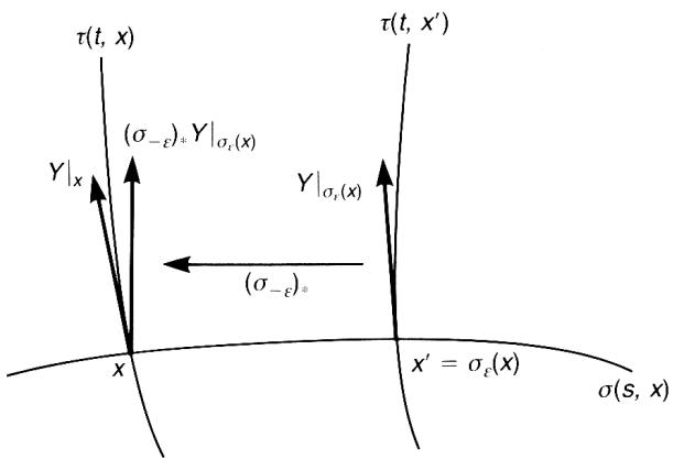
Figure 5.12. To compare a vector $Y{|}_x$ with $Y{|}_{{\sigma }_{\epsilon }(x)}$ , the latter must be transported back to $x$ by the differential map $({\sigma }_{-\epsilon }{)}_{\ast }$ .

$${\mathcal{L}}_{X}Y=\underset{\epsilon \to 0}{\lim }\frac{1}{\epsilon }[({\sigma }_{-\epsilon }{)}_{\ast }Y{|}_{{\sigma }_{\epsilon }(x)}-Y{|}_x].\text{\hspace{1em}(5.47)}$$

Exercise 5.8

Show that ${\mathcal{L}}_{X}Y$ is also written as

$$\begin{array}{rl}{\mathcal{L}}_{X}Y& =\underset{\epsilon \to 0}{\lim }\frac{1}{\epsilon }[Y{|}_x-({\sigma }_{\epsilon }{)}_{\ast }Y{|}_{{\sigma }_{-\epsilon }(x)}]\\ & =\underset{\epsilon \to 0}{\lim }\frac{1}{\epsilon }[Y{|}_{{\sigma }_{\epsilon }(x)}-({\sigma }_{\epsilon }{)}_{\ast }Y{|}_x].\end{array}$$

Let $(U,\phi )$ be a chart with the coordinates $x$ and let $X=X^{\mu }\partial /\partial x^{\mu }$ and $Y=Y^{\mu }\partial /\partial x^{\mu }$ be vector fields defined on $U$ . Then ${\sigma }_{\epsilon }(x)$ has the coordinates $x^{\mu }+\epsilon X^{\mu }(x)$ and

$$\begin{array}{rl}Y{|}_{{\sigma }_{\epsilon }(x)}& =Y^{\mu }\left(x^v+\epsilon X^v(x)\right)e_{\mu }{|}_{x+\epsilon X}\\ & \simeq \left[Y^{\mu }(x)+\epsilon X^{\mu }(x){\partial }_v{Y}^{\mu }(x)\right]e_{\mu }{|}_{x+\epsilon X}\end{array}$$

where $\{e_{\mu }\}=\{\partial /\partial x^{\mu }\}$ is the coordinate basis and ${\partial }_{\nu }\equiv \partial /\partial x^{\nu }$ . If we map this vector defined at ${\sigma }_{\epsilon }(x)$ to $x$ by $({\sigma }_{-\epsilon }{)}_{\ast }$ , we obtain

$$\begin{array}{rl}& [Y^{\mu }(x)+\epsilon X^{\lambda }(x){\partial }_{\lambda }{Y}^{\mu }(x)]{\partial }_{\mu }[x^{\nu }-\epsilon X^{\nu }(x)]e_{\nu }{|}_x\\ & =[Y^{\mu }(x)+\epsilon X^{\lambda }(x){\partial }_{\lambda }{Y}^{\mu }(x)][{\delta }_{\mu }^{\nu }-\epsilon {\partial }_{\mu }{X}^{\nu }(x)]e_{\nu }{|}_x\\ & =Y^{\mu }(x)e_{\mu }{|}_x+\epsilon \left[X^{\mu }(x){\partial }_{\mu }{Y}^{\nu }(x)-Y^{\mu }(x){\partial }_{\mu }{X}^{\nu }(x)\right]e_{\nu }{|}_x+O\left({\epsilon }^2\right).\end{array}\text{\hspace{1em}(5.48)}$$

From (5.47) and (5.48), we find that

$${\mathcal{L}}_{X}Y=\left(X^{\mu }{\partial }_{\mu }{Y}^{\nu }-Y^{\mu }{\partial }_{\mu }{X}^{\nu }\right)e_{\nu }.\text{\hspace{1em}(5.49a)}$$

Exercise 5.9

Let $X=X^{\mu }\partial /\partial x^{\mu }$ and $Y=Y^{\mu }\partial /\partial x^{\mu }$ be vector fields in $M$ . Define the Lie bracket $[X,Y]$ by

$$[X,Y]f=X[Y[f]]-Y[X[f]]\text{\hspace{1em}(5.50)}$$

where $f\in \mathcal{F}(M)$ . Show that $[X,Y]$ is a vector field given by

$$\left(X^{\mu }{\partial }_{\mu }{Y}^{\nu }-Y^{\mu }{\partial }_{\mu }{X}^{\nu }\right)e_{\nu }.$$

This exercise shows that the Lie derivative of $Y$ along $X$ is

$${\mathcal{L}}_{X}Y=[X,Y].\text{\hspace{1em}(5.49b)}$$

[Remarks: Note that neither $XY$ nor $YX$ is a vector field since they are second-order derivatives. The combination $[X,Y]$ is, however, a first-order derivative and indeed a vector field.]

Exercise 5.10

Show that the Lie bracket satisfies

(a) bilinearity

$$[X,c_1{Y}_1+c_2{Y}_2]=c_1[X,Y_1]+c_2[X,Y_2]$$

$$[c_1{X}_1+c_2{X}_2,Y]=c_1[X_1,Y]+c_2[X_2,Y]$$

for any constants $c_1$ and $c_2$ ,

(b) skew-symmetry

$$[X,Y]=-[YX]$$

(c) the Jacobi identity

$$[[X,Y],Z]+[[Z,X],Y]+[[Y,Z],X]=0.$$

Exercise 5.11

(a) Let $X,Y\in \mathcal{X}(M)$ and $f\in \mathcal{F}(M)$ . Show that

$${\mathcal{L}}_{fX}Y=f[X,Y]-Y[f]X\text{\hspace{1em}(5.51a)}$$

$${\mathcal{L}}_X(fY)=f[X,Y]+X[f]Y.\text{\hspace{1em}(5.51b)}$$

(b) Let $X,Y\in \mathcal{X}(M)$ and $f:M\to N$ . Show that

$$f_{\ast }[X,Y]=\left[f_{\ast }X,f_{\ast }Y\right].\text{\hspace{1em}(5.52)}$$

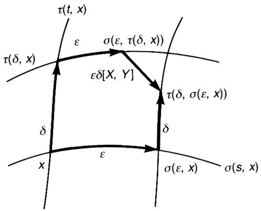
Geometrically, the Lie bracket shows the non-commutativity of two flows. This is easily observed from the following consideration. Let $\sigma (s,x)$ and $\tau (t,x)$ be two flows generated by vector fields $X$ and $Y$ , as before, see figure 5.13. If we move by a small parameter distance $\epsilon$ along the flow $\sigma$ first, then by $\delta$ along $\tau$ , we shall be at the point whose coordinates are

Figure 5.13. A Lie bracket $[X,Y]$ measures the failure of the closure of the parallelogram.

$$\begin{array}{rl}& {\tau }^{\mu }(\delta ,\sigma (\epsilon ,x))\simeq {\tau }^{\mu }(\delta ,x^v+\epsilon X^v(x))\\ & \simeq x^{\mu }+\epsilon X^{\mu }(x)+\delta Y^{\mu }\left(x^v+\epsilon X^v(x)\right)\\ & \simeq x^{\mu }+\epsilon X^{\mu }(x)+\delta Y^{\mu }(x)+\epsilon \delta X^v(x){\partial }_v{Y}^v(x).\end{array}$$

If, however, we move by $\delta$ along $\tau$ first, then by $\epsilon$ along $\sigma$ , we will be at the point

$$\begin{array}{rl}& {\sigma }^{\mu }(\epsilon ,\tau (\delta ,x))\simeq {\sigma }^{\mu }(\epsilon ,x^v+\delta Y^v(x))\\ & \simeq x^{\mu }+\delta Y^{\mu }(x)+\epsilon X^{\mu }\left(x^v+\delta Y^v(x)\right)\\ & \simeq x^{\mu }+\delta Y^{\mu }(x)+\epsilon X^{\mu }(x)+\epsilon \delta Y^v(x){\partial }_v{X}^{\mu }(x).\end{array}$$

The difference between the coordinates of these two points is proportional to the Lie bracket,

$${\tau }^{\mu }(\delta ,\sigma (\epsilon ,x))-{\sigma }^{\mu }(\epsilon ,\tau (\delta ,x))=\epsilon \delta [X,Y{]}^{\mu }.$$

The Lie bracket of $X$ and $Y$ measures the failure of the closure of the parallelogram in figure 5.13. It is easy to see ${\mathcal{L}}_{X}Y=[X,Y]=0$ if and only if

$$\sigma (s,\tau (t,x))=\tau (t,\sigma (s,x)).\text{\hspace{1em}(5.53)}$$

We may also define the Lie derivative of a one-form $\omega \in {\Omega }^1(M)$ along $X\in \mathcal{X}(M)$ by

$${\mathcal{L}}_X\omega \equiv \underset{\epsilon \to 0}{\lim }\frac{1}{\epsilon }[({\sigma }_{\epsilon }{)}^{\ast }\omega {|}_{{\sigma }_{\epsilon }(x)}-\omega {|}_x]\text{\hspace{1em}(5.54)}$$

where $\omega {|}_x\in T_x^{\ast }M$ is $\omega$ at $x$ . Put $\omega ={\omega }_{\mu }\mathrm{d}{x}^{\mu }$ . Repeating a similar analysis as before, we obtain

$${{\left({\sigma }_{\epsilon }\right)}^{\ast }\omega |}_{{\sigma }_{\epsilon }(x)}={\omega }_{\mu }(x)d{x}^{\mu }+\epsilon \left[X^v(x){\partial }_v{\omega }_{\mu }(x)+{\partial }_{\mu }{X}^v(x){\omega }_v(x)\right]d{x}^{\mu }$$

which leads to

$${\mathcal{L}}_X\omega =\left(X^{\nu }{\partial }_{\nu }{\omega }_{\mu }+{\partial }_{\mu }{X}^{\nu }{\omega }_{\nu }\right)d{x}^{\mu }.\text{\hspace{1em}(5.55)}$$

Clearly ${\mathcal{L}}_X\omega \in T_x^{\ast }(M)$ , since it is a difference of two one-forms at the same point $x$ .

The Lie derivative of $f\in \mathcal{F}(M)$ along a flow ${\sigma }_s$ generated by a vector field $X$ is

$$\begin{array}{rl}& {\mathcal{L}}_{X}f\equiv \underset{\epsilon \to 0}{\lim }\frac{1}{\epsilon }[f({\sigma }_{\epsilon }(x))-f(x)]\\ & =\underset{\epsilon \to 0}{\lim }\frac{1}{\epsilon }[f(x^{\mu }+\epsilon X^{\mu }(x))-f(x^{\mu })]\\ & =X^{\mu }(x)\frac{\partial f}{\partial x^{\mu }}=X[f]\end{array}\text{\hspace{1em}(5.56)}$$

which is the usual directional derivative of $f$ along $X$ .

The Lie derivative of a general tensor is obtained from the following proposition.

Proposition 5.1

The Lie derivative satisfies

$${\mathcal{L}}_X\left(t_1+t_2\right)={\mathcal{L}}_X{t}_1+{\mathcal{L}}_X{t}_2\text{\hspace{1em}(5.57a)}$$

where $t_1$ and $t_2$ are tensor fields of the same type and

$${\mathcal{L}}_X\left(t_1\otimes t_2\right)=\left({\mathcal{L}}_X{t}_1\right)\otimes t_2+t_1\otimes \left({\mathcal{L}}_X{t}_2\right)\text{\hspace{1em}(5.57b)}$$

where $t_1$ and $t_2$ are tensor fields of arbitrary types.

Proof

(a) is obvious. Rather than giving the general proof of (b), which is full of indices, we give an example whose extension to more general cases is trivial. Take $Y\in \mathcal{X}(M)$ and $\omega \in {\Omega }^1(M)$ and construct the tensor product $Y\otimes \omega$ . Then $(Y\otimes \omega ){|}_{{\sigma }_{\epsilon }(x)}$ is mapped onto a tensor at $x$ by the action of $({\sigma }_{-\epsilon }{)}_{\ast }\otimes ({\sigma }_{\epsilon }{)}^{\ast }$ :

$$[({\sigma }_{-\epsilon }{)}_{\ast }\otimes ({\sigma }_{\epsilon }{)}^{\ast }](Y\otimes \omega ){|}_{{\sigma }_{\epsilon }(X)}=[({\sigma }_{-\epsilon }{)}_{\ast }Y\otimes ({\sigma }_{\epsilon }{)}^{\ast }\omega ]{|}_X.$$

Then there follows (the Leibnitz rule):

$$\begin{array}{rl}{\mathcal{L}}_X(Y\otimes \omega )& =\underset{\epsilon \to 0}{\lim }\frac{1}{\epsilon }[\left\{{\left({\sigma }_{-\epsilon }\right)}_{\ast }Y\otimes {\left({\sigma }_{\epsilon }\right)}^{\ast }\omega \right\}{|}_x-(Y\otimes \omega ){|}_x]\\ & =\underset{\epsilon \to 0}{\lim }\frac{1}{\epsilon }[({\sigma }_{-\epsilon }{)}_{\ast }Y\otimes \left\{{\left({\sigma }_{\epsilon }\right)}^{\ast }\omega -\omega \right\}+\left\{{\left({\sigma }_{-\epsilon }\right)}_{\ast }Y-Y\right\}\otimes \omega ]\\ & =Y\otimes ({\mathcal{L}}_X\omega )+({\mathcal{L}}_{X}Y)\otimes \omega .\end{array}$$

Extensions to more general cases are obvious.

This proposition enables us to calculate the Lie derivative of a general tensor field. For example, let $t=t_{\mu }^{\nu }\mathrm{d}{x}^{\mu }\otimes e_{\nu }\in {\mathcal{T}}_1^1(M)$ . Proposition 5.1 gives

$${\mathcal{L}}_{X}t=X\left[t_{\mu }^v\right]d{x}^{\mu }\otimes e_v+t_{\mu }^v\left({\mathcal{L}}_{X}d{x}^{\mu }\right)\otimes e_v+t_{\mu }^{v}d{x}^{\mu }\otimes \left({\mathcal{L}}_X{e}_v\right).$$

Exercise 5.12

Let $t$ be a tensor field. Show that

$${\mathcal{L}}_{[X,Y]}t={\mathcal{L}}_X{\mathcal{L}}_{Y}t-{\mathcal{L}}_Y{\mathcal{L}}_{X}t.\text{\hspace{1em}(5.58)}$$

来源与版本

正文：英文 · OCR 机器稿 · 待校对

核对状态：OCR 机器稿 · 待校对

原书 PDF

来源版本：second-edition-local

来源 PDF SHA-256：fcd24c3371d092a8c699ccf5cf0765462924b6c48412804231076e8084b1940d

OCR 来源 SHA-256：0b6324f01172a3548cd34382e82fd8bfae574602b6b2cfaa357ba96bc2c35478

OCR 产物 SHA-256：28e1671b2f931833602060b4f9f4e242bc60cdc164d2e7f44aff27181497fc0d