4.3 Linear ordinary differential equations

中文

While no techniques exist for solving general differential equations, systems of linear ordinary differential equations with constant coefficients are completely solvable with the help of the Jordan form. Such systems can be written in the form

$$\dot{\mathbf{x}}\equiv \frac{\mathrm{d}\mathbf{x}}{\mathrm{d}t}=\mathsf{Ax},\text{\hspace{1em}(4.27)}$$

where $\mathbf{x}(t)$ is an $n\times 1$ column vector and $A$ an $n\times n$ matrix of real constants. Initially it is best to consider this as an equation in complex variables $x$, even though we may only be seeking real solutions. Greater details of the following discussion, as well as applications to non-linear differential equations, can be found in [4, 5].

Try for a solution of Eq. (4.27) in exponential form

$$\mathbf{x}(t)={\mathrm{e}}^{\mathsf{A}t}{\mathbf{x}}_0,\text{\hspace{1em}(4.28)}$$

where ${\mathbf{X}}_0$ is an arbitrary constant vector, and the exponential of a matrix is defined by the convergent series

$$e^S=I+S+\frac{S^2}{2!}+\frac{S^3}{3!}+\dots \text{\hspace{1em}(4.29)}$$

If $S$ and $T$ are two commuting matrices, $\mathsf{ST}=\mathsf{TS}$ , it then follows just as for real or complex scalars that ${\mathrm{e}}^{\mathsf{ST}}={\mathrm{e}}^{\mathsf{S}}{\mathrm{e}}^{\mathsf{T}}$

The initial value at $t=0$ of the solution given by Eq. (4.28) is clearly $\mathbf{x}(0)={\mathbf{x}}_0$ . If $P$ is any invertible $n\times n$ matrix, then $\mathbf{y}=\mathsf{P}\mathbf{x}$ satisfies the differential equation

$$\dot{\mathbf{y}}={\mathsf{A}}^{\prime }\mathbf{y}\text{ where }{\mathsf{A}}^{\prime }={\mathsf{PAP}}^{-1},$$

and gives rise to the solution

$$\mathbf{y}={\mathrm{e}}^{{\mathsf{A}}^{\prime }t}{\mathbf{y}}_0\text{where}{\mathbf{y}}_0={\mathsf{Px}}_0.$$

If $P$ is chosen such that ${\mathsf{A}}^{\prime }$ has the Jordan form

$${\mathsf{A}}^{\prime }=\left(\begin{array}{ccc}{\lambda }_1\mathsf{I}+{\mathsf{N}}_{11}& & \\ & \ddots & \\ & & {\lambda }_m\mathsf{I}+{\mathsf{N}}_{m{r}_m}\end{array}\right)$$

where the ${\mathsf{N}}_{ij}$ are nilpotent matrices then, since ${\lambda }_i\mathsf{I}$ commutes with $N_{ij}$ for every $i,j,$ , the exponential term has the form

$${\mathrm{e}}^{{\mathsf{A}}^{\prime }t}=\left(\begin{array}{ccc}{\mathrm{e}}^{{\lambda }_{1}t}{\mathrm{e}}^{{\mathsf{N}}_{11}t}& & \\ & \ddots & \\ & & {\mathrm{e}}^{{\lambda }_{m}t}{\mathrm{e}}^{{\mathsf{N}}_{mrm}t}\end{array}\right).$$

If $N$ is a Jordan matrix of order $k\times k$ having 1’s along the superdiagonal as in Eq. (4.25), then ${\mathsf{N}}^2$ has 1’s in the next diagonal out and each successive power of $N$ pushes this diagonal of 1’s one place further until ${\mathsf{N}}^k$ vanishes altogether,

$${\mathsf{N}}^2=\left(\begin{array}{ccccc}0& 0& 1& 0& \dots \\ 0& 0& 0& 1& \dots \\ & & & \ddots & \\ 0& 0& 0& \dots & 0\end{array}\right),\dots ,{\mathsf{N}}^{k-1}=\left(\begin{array}{ccccc}0& 0& 0& \dots & 1\\ 0& 0& 0& \dots & 0\\ & & & \ddots & \\ & & & \dots & 0\end{array}\right),{\mathsf{N}}^k=\mathsf{O}.$$

Hence

$${\mathrm{e}}^{\mathsf{N}t}=\left(\begin{array}{ccccc}1& t& \frac{t^2}{2}& \dots & \frac{t^{k-1}}{(k-1)!}\\ 0& 1& t& \dots & \\ & & & \ddots & \\ 0& 0& & \dots & 1\end{array}\right),$$

and the solution Eq. (4.28) can be expressed as a linear supposition of solutions of the form

$${\mathbf{x}}_r(t)={\mathbf{w}}_r(t){\mathrm{e}}^{{\lambda }_{i}t}\text{\hspace{1em}(4.30)}$$

where

$${\mathbf{w}}_r(t)=\frac{t^{r-1}}{(r-1)!}{\mathbf{h}}_1+\frac{t^{r-2}}{(r-2)!}{\mathbf{h}}_2+\cdots +t{\mathbf{h}}_{r-1}+{\mathbf{h}}_r.\text{\hspace{1em}(4.31)}$$

If $A$ is a real matrix then the matrices $P$ and ${\mathsf{A}}^{\prime }$ are in general complex, but given real initial values ${\mathbf{X}}_0$ the solution having these values at $t=0$ is

$$\mathbf{x}={\mathsf{P}}^{-1}\mathbf{y}={\mathsf{P}}^{-1}{\mathrm{e}}^{{\mathsf{A}}^{\prime }t}\mathsf{P}{\mathbf{x}}_0,$$

which must necessarily be real by the existence and uniqueness theorem of ordinary differ ential equations. Alternatively, for $A$ real, both the real and imaginary parts of any complex solution $\mathbf{x}(t)$ are solutions of the linear differential equation Eq. (4.27), which may be separated by the identity

$${\mathrm{e}}^{\lambda t}=\cos \lambda t+i\sin \lambda t.$$

Two-dimensional autonomous systems

Consider the special case of a planar (two-dimensional) system Eq. (4.27) having constant coefficients, known as an autonomous system,

$$\dot{\mathbf{x}}=\mathsf{A}\mathbf{x}\text{ where }\mathsf{A}=\left(\begin{array}{cc}{a}_{11}& a_{12}\\ a_{21}& a_{22}\end{array}\right),\mathbf{x}=\left(\genfrac{}{}{0ex}{}{x_1}{x_2}\right).$$

Both the matrix $A$ and vector $x$ are assumed to be real. A critical point ${\mathbf{X}}_0$ refers to any constant solution $\mathbf{X}={\mathbf{X}}_0$ of Eq. (4.27). The analysis of autonomous systems breaks up into a veritable zoo ofcases and subcases. We consider the case where the matrix $A$ is non-singular, for which the only critical point is ${\mathbf{x}}_0=0$ . Both eigenvalues ${\lambda }_1$ and ${\lambda }_2$ are $\ne 0$ , and the following possibilities arise.

(1) $|{\lambda }_1\ne {\lambda }_2$ and both eigenvalues are real. In this case the eigenvectors ${\mathbf{h}}_1$ and ${\mathbf{h}}_2$ form a basis of ${\mathbb{R}}^2$ and the general solution is

$$\mathbf{x}=c_1{\mathrm{e}}^{{\lambda }_{1}t}{\mathbf{h}}_1+c_2{\mathrm{e}}^{{\lambda }_{2}t}{\mathbf{h}}_2.$$

(1a) If ${\lambda }_2<{\lambda }_1<0$ the critical point is called a stable node.

(1b) If ${\lambda }_2>{\lambda }_1>0$ the critical point is called an unstable node.

(1c) If ${\lambda }_2<0<{\lambda }_1$ the critical point is called a saddle point.

These three cases are shown in Fig. 4.1, after the basis of the vector space axes has been transformed to lie along the vectors ${\mathbf{h}}_i$

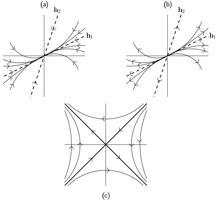Figure 4.1 (a) Stable node, (b) unstable node, (c) saddle point

(2) ${\lambda }_1=\lambda ,{\lambda }_2=\overline{\lambda }$ where $\lambda$ is complex. The eigenvectors are then complex conjugate to each other since $A$ is a real matrix,

$$\mathbf{Ah}=\lambda \mathbf{h}\Rightarrow \mathbf{A}\overline{\mathbf{h}}=\overline{\lambda }\mathbf{h},$$

and the arbitrary real solution is

$$\mathbf{x}=c{\mathrm{e}}^{\lambda t}\mathbf{h}+\overline{c}{\mathrm{e}}^{\overline{\lambda }t}\overline{\mathbf{h}}.$$

If we set

$$\mathbf{h}=\frac{1}{2}({\mathbf{h}}_1-i{\mathbf{h}}_2),\lambda =\mu +i\nu ,c=R{e}^{i\alpha }$$

where ${\mathbf{h}}_1,{\mathbf{h}}_2,\mu ,\nu ,R>0$ and $\alpha$ are all real quantities, then the solution $x$ has the form

$$\mathbf{x}=R{\mathrm{e}}^{\mu t}\left(\cos (\nu t+\alpha ){\mathbf{h}}_1+\sin (\nu t+\alpha ){\mathbf{h}}_2\right).$$

(2a) $\mu <0:$ This is a logarithmic spiral approaching the critical point $\mathbf{x}=0$ as $t\to \infty$ , and is called a stable focus.

(2b) $\mu >0;$ Again the solution is a logarithmic spiral but arising from the critical point $\mathbf{x}=0$ as $t\to -\infty ,$ , called an unstable focus.

(2c) $\mu =0;$ With respect to the basis ${\mathbf{h}}_1,{\mathbf{h}}_2$ , the solution is a set of circles about the origin.

When the original basis ${\mathbf{e}}_1=\left(\genfrac{}{}{0ex}{}{1}{0}\right),{\mathbf{e}}_2=\left(\genfrac{}{}{0ex}{}{0}{1}\right)$ is used, the solutions are a set ofellipses and the critical point is called a vortex point.

These solutions are depicted in Fig. 4.2.

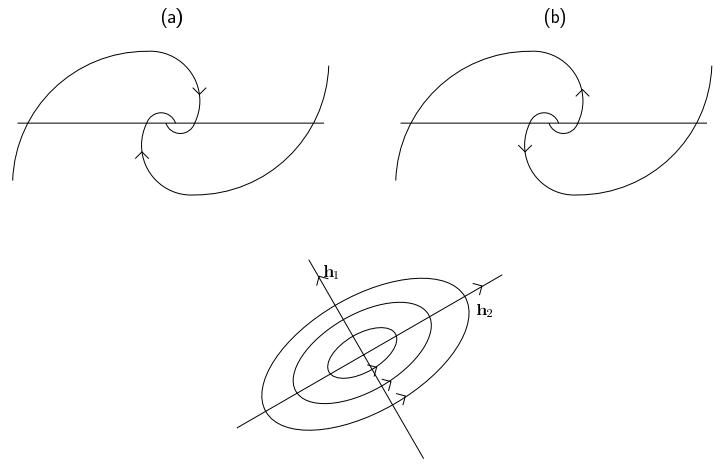Figure 4.2 (a) Stable focus, (b) unstable focus, (c) vortex point

Problems

Problem 4.5

Verify that Eq. (4.30), Eq. (4.31) is a solution of ${\dot{\mathbf{x}}}_r=\mathsf{A}{\mathbf{x}}_r(t)$ provided

$$\begin{array}{c}{\mathbf{Ah}}_1={\lambda }_i{\mathbf{h}}_1\\ {\mathbf{Ah}}_2={\lambda }_i{\mathbf{h}}_2+{\mathbf{h}}_1\\ ⋮\\ {\mathbf{Ah}}_r={\lambda }_i{\mathbf{h}}_r+{\mathbf{h}}_{r-1}\end{array}$$

where ${\lambda }_i$ is an eigenvalue of $A$.

Problem 4.6

Discuss the remaining cases for two-dimensional autonomous systems: (a) ${\lambda }_1={\lambda }_2=$ $\lambda \ne 0$ and (i) two distinct eigenvectors ${\mathbf{h}}_1$ and ${\mathbf{h}}_2,$ , (ii) only one eigenvecto ${\mathbf{h}}_1;(\mathbf{b})$ $A$ a singular matrix. Sketch the solutions in all instances.

Problem 4.7

Classify all three-dimensional autonomous systems of linear differential equations having constant coefficients.