14.1 Basic concepts

中文

Photon polarization experiments

To understand how quantum mechanics works, we look at the outcome of a number of Gedanken experiments involving polarized light beams. Typically, a monochromatic plane wave solution or Maxwell equations (see Problem 9.23) has electric field

$$\mathbf{E}\propto \mathrm{Re}\left(\alpha {\mathbf{e}}_x+\beta {\mathbf{e}}_y\right){\mathrm{e}}^{i(kz-\omega t)}$$

where ${\mathbf{e}}_x$ and ${\mathbf{e}}_y$ are the unit vectors in the $x$- and $y$-directions and $\alpha$ and $\beta$ are complex numbers such that

$$|\alpha {|}^2+|\beta {|}^2=1.$$

When $\alpha /\beta$ is real we have a linearly polarized wave, as for example

$$\mathbf{E}\propto \frac{1}{\sqrt{2}}({\mathbf{e}}_x+{\mathbf{e}}_y){\mathrm{e}}^{i(kz-\omega t)}.$$

If $b=\pm ia=\pm i/\sqrt{2}$ the wave is circularly polarized; the sign is said to be right cir cularly polarized, and the sign is left circularly polarized. In all other cases it is said to be elliptically polarized. If we pass a polarized beam through a polarizer with axis of polarization ${\mathbf{e}}_x$ , then the beam is reduced in intensity by the factor $|a{|}^2$ and the emergen beam is ${\mathbf{e}}_x$ -polarized. Thus, if the resultant beam is passed through another ${\mathbf{e}}_x$ -polarizer it will be 100% transmitted, while if it is passed through an ${\mathbf{e}}_y-\mathrm{polarizer}$ it will be totally absorbed and nothing will come through. This is the classical situation.

As was discovered by Planck and Einstein at the turn of the twentieth century, light beams come in discrete packets called photons, having energy $E=h\nu =\hslash \omega$ where $h\approx 6.625\times 10^{-27}\mathrm{g}{\mathrm{cm}}^2{\mathrm{s}}^{-1}$ is Planck’s constant and $\hslash =h/2\pi$ . What happens if we send the beams through the polarizers one photon at a time? Since the frequency of each photon is unchanged it emerges with the same energy, and since the intensity of the beam is related to the energy, it must mean that the number of photons is reduced. However, the most obvious conclusion that the beam consists of a mixture of photons consisting of a fraction $|\alpha {|}^2$ polarized in the ${\mathbf{e}}_x$ -direction and $|\beta {|}^2$ in the ${\mathbf{e}}_{\nu }$ -direction will not stand up to scrutiny. For, if a beam with $\alpha =\beta =1/\sqrt{2}$ were passed through a polarizer designed to only transmit waves linearly polarized in the $({\mathbf{e}}_x+{\mathbf{e}}_y)/\sqrt{2}$ direction, then it should be 100% transmitted. However, on the mixture hypothesis only half the ${\mathbf{e}}_x$ -polarized photons should get through, and half the ${\mathbf{e}}_y-\mathsf{polarized}$ photons, leaving a total fraction $\begin{array}{r}\frac{1}{2}\cdot \frac{1}{2}+\frac{1}{2}\cdot \frac{1}{2}=\frac{1}{2}\end{array}$ being transmitted.

In quantum mechanics it is proposed that each photon is a ‘complex superposition $\alpha {\mathbf{e}}_x+\beta {\mathbf{e}}_y$ of the two polarization states ${\mathbf{e}}_x$ and ${\mathbf{e}}_y$ . The probability of transmission by an ${\mathbf{e}}_x$ -polarizer is given by $|\alpha {|}^2$ , while the probability of transmission by an ${\mathbf{e}}_y$ -polarizer is $|\beta {|}^2$ The effect of the ${\mathbf{e}}_x$ -polarizer is essentially to ‘collapse’ the photon into an ${\mathbf{e}}_x$ -polarized state. The polarizer can be regarded both as a measuring device or equally as a device fo preparing photons in an ${\mathbf{e}}_x-\mathrm{polarized}$ state. If used as a measuring device it returns the value 1 ifthe photon is transmitted, or 0 if not – in either case the act of measurement has changed the state of the photon being measured.

An interesting arrangement to illustrate the second point of view is shown in Fig. 14.1. Consider a beam of photons incident on an ${\mathbf{e}}_x-\mathrm{polarizer},$ followed by an ${\mathbf{e}}_y$ -polarizer; the net result is that no photons come out of the second polarizer. Now introduce a polarizer for the direction $(1/\sqrt{2})({\mathbf{e}}_x+{\mathbf{e}}_y)$ – in other words a device that should block some of the photons between the two initial polarizers. If the mixture theory were correct, it is inconceivable that this could increase transmission. Yet the reality is that half the photons emerge from this intermediary polarizer with polarization $(1/\sqrt{2})({\mathbf{e}}_x+{\mathbf{e}}_y)$ ), and a further half of these, namely a quarter in all, are now transmitted by the ${\mathbf{e}}_y-\mathrm{polarizer}.$

How can we find the transmission probability of a polarized state $A$ with respect to an arbitrary polarization direction $B$? The following argument is designed to be motivational rather than rigorous. Let $\mathbf{A}=\alpha {\mathbf{e}}_x+\beta {\mathbf{e}}_y$ , where $\alpha$ and $\beta$ are complex numbers subject to $|\alpha {|}^2+|\beta {|}^2=1$ . We write $\alpha =⟨{\mathbf{e}}_x\mid \mathbf{A}⟩$ , called the amplitude for ${\mathbf{e}}_x$ -transmission of an

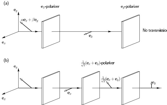
Figure 14.1 Photon polarization experiment

$A$-polarized photon. It is a complex number having no obvious physical interpretation of itself, but its magnitude square $|\alpha {|}^2$ is the probability of transmission by an ${\mathbf{e}}_x$ -polarizer. Similarly $\beta =⟨{\mathbf{e}}_y\mid \mathbf{A}⟩$ is the amplitude for ${\mathbf{e}}_y$ -transmission, and $|\beta {|}^2$ the probability of transmission by an ${\mathbf{e}}_y-\mathrm{polarizer}.$ . What is the polarization $A^{\perp }$ such that a polarizer of this type allows for no transmission, $⟨{\mathbf{A}}^{\perp }|\mathbf{A}⟩=0?$ For linearly polarized waves with $\alpha$ and $\beta$ both real we expect it to be geometrically orthogonal, ${\mathbf{A}}^{\perp }=\beta {\mathbf{e}}_x-\alpha {\mathbf{e}}_y$ . For circularly polarized waves, the orthogonal ‘direction’ is the opposite circular sense. Hence

$$\frac{1}{\sqrt{2}}{\left({\mathbf{e}}_x\pm i{\mathbf{e}}_y\right)}^{\perp }=\frac{1}{\sqrt{2}}\left({\mathbf{e}}_x\mp i{\mathbf{e}}_y\right)\equiv \mp \frac{1}{\sqrt{2}}\left(i{\mathbf{e}}_x-{\mathbf{e}}_y\right)$$

since phase factors such as $i$ are irrelevant. In the general elliptical case we might guess tha ${\mathbf{A}}^{\perp }=\overline{\beta }{\mathbf{e}}_x-\overline{\alpha }{\mathbf{e}}_y$ , since it reduces to the correct answer for linear and circular polarization. Solving for ${\mathbf{e}}_x$ and ${\mathbf{e}}_y$ we have

$${\mathbf{e}}_x=\overline{\alpha }\mathbf{A}+\beta {\mathbf{A}}^{\perp },{\mathbf{e}}_y=\overline{\beta }\mathbf{A}-\alpha {\mathbf{A}}^{\perp }.$$

Let $\mathbf{B}=\gamma {\mathbf{e}}_x+\delta {\mathbf{e}}_y$ be any other polarization, then substituting for ${\mathbf{e}}_x$ and ${\mathbf{e}}_y$ gives

$$\mathbf{B}=(\gamma \overline{\alpha }+\delta \overline{\beta })\mathbf{A}+(\gamma \beta -\alpha \delta ){\mathbf{A}}^{\perp }.$$

Setting $B=A$ gives the normalization condition $|\alpha {|}^2+|\beta {|}^2=1$ . Hence, since $⟨\mathbf{A}|\mathbf{A}⟩=1$ (transmission probability of 1),

$$⟨\mathbf{B}|\mathbf{A}⟩=(\gamma \overline{\alpha }+\delta \overline{\beta })=\overline{⟨\mathbf{A}|\mathbf{B}⟩}.$$

Other systems such as the Stern–Gerlach experiment, in which an electron of magnetic moment $\mu$ is always deflected in a magnetic field $H$ in just two directions, exhibit a completely analogous formalism. The conclusion is that the quantum mechanical states of a system form a complex vector space with inner product $⟨\varphi \mid \psi ⟩$ satisfying the usua

conditions

$$⟨\varphi |\alpha {\psi }_1+\beta {\psi }_2⟩=\alpha ⟨\varphi |{\psi }_1⟩+\beta ⟨\varphi |{\psi }_2⟩\text{ and }⟨\varphi |\psi ⟩=\overline{⟨\psi |\varphi ⟩}.$$

The probability of obtaining a value corresponding to $\varphi$ in a measurement is

$$P(\varphi ,\psi )=|⟨\varphi |\psi ⟩{|}^2.$$

As will be seen, states are in fact normalized to $⟨\psi |\psi ⟩=1$ , so that only linear combinations $\alpha {\psi }_1+\beta {\psi }_2$ with $|\alpha {|}^2+|\beta {|}^2=1$ are permitted.

The Hilbert space of states

We will now assume that every physical system corresponds to a separable Hilbert space , representing all possible states of the system. The Hilbert space may be finite dimensional, as for example the states of polarization of a photon or electron, but often it is infinite dimensional. A state of the system is represented by a non-zero vector $\psi \in \mathcal{H}.$ , but this correspondence is not one-to-one, as any two vectors $\psi$ and ${\psi }^{\prime }$ that are proportional through a non-zero complex factor, ${\psi }^{\prime }=\lambda \psi$ where $\lambda \in \mathbb{C}$ , will be assumed to represent identical states. In other words, a state is an equivalence class or ray of vectors $[\psi ]$ all related by proportionality. A state may be represented by any vector from the class, and it is standard to select a representative having unit norm $\Vert \psi \Vert =1$ . Even this restriction does not uniquely define a vector to represent the state, as any other vector ${\psi }^{\prime }=\lambda \psi$ with $|\lambda |=1$ will also satisfy the unit norm condition. The angular freedom, $\lambda ={\mathrm{e}}^{ic}$ , is sometimes referred to as the phase of the state vector. Phase is only significant in a relative sense; for example, $\psi +{\mathrm{e}}^{ic}\varphi$ is in general a different state to $\psi +\varphi$ , but ${\mathsf{e}}^{ic}(\psi +\varphi )$ is not.

In this chapter we will adopt Dirac’s bra-ket notation which, though slightly quirky, has largely become the convention of choice among physicists. Vectors $\psi \in \mathcal{H}$ are written as kets $|\psi ⟩$ and one makes the identification $|\lambda \psi ⟩=\lambda |\psi ⟩$ . By the Riesz representation theorem 13.10, to each linear functional $f:\mathcal{H}\to \mathbb{C}$ there corresponds a unique vector $\varphi \equiv |\varphi ⟩\in \mathcal{H}$ such that $f(\psi )=⟨\varphi |\psi ⟩$ . In Dirac’s terminology the linear functional is referred to as a bra, written $⟨\varphi |$ . The relation between bras and kets is antilinear,

$$⟨\lambda \psi +\varphi |=\overline{\lambda }⟨\psi |+⟨\varphi |.$$

In Dirac’s notation it is common to think of a linear operator $(A,D_A)$ as acting to the lef on kets (vectors), while acting to the right on bras (linear functionals):

$$A|\psi ⟩\equiv |A\psi ⟩,$$

and if $\varphi \in D_A$

$$⟨\varphi |A\equiv ⟨A^{\ast }\varphi |.$$

The following notational usages for the matrix elements of an operator between two vectors are all equivalent:

$$⟨\varphi |A|\psi ⟩\equiv ⟨\varphi |A\psi ⟩=⟨A^{\ast }\varphi |\psi ⟩=\overline{⟨\psi |A^{\ast }\varphi ⟩}=\overline{⟨\psi |A^{\ast }|\varphi ⟩}.$$

$\mathrm{If}|e_i$ is an o.n. basis of kets in a separable Hilbert space then we may write

$$A|e_j⟩=\sum _i{a}_{ij}|e_i⟩\text{ where }{a}_{ij}=⟨e_i|A|e_j⟩.$$

Observables

In classical mechanics,physical observables refer to quantities such as position, momentum, energy or angular momentum, which are real numbers or real multicomponented objects. In quantum mechanics observables are represented by self-adjoint operators on the Hilbert space of states. We first consider the case where $A$ is a hermitian operator (bounded and continuous). Such an observable is said to be complete if the corresponding hermitian operator $A$ is complete, so that there is an orthonormal basis made up of eigenvectors $|{\psi }_1⟩,|{\psi }_2⟩,...$ . such that

$$A|{\psi }_n⟩={\alpha }_n|{\psi }_n⟩\text{ where }⟨{\psi }_m|{\psi }_n⟩={\delta }_{mn}.\text{\hspace{1em}(14.1)}$$

The result of measuring a complete observable is always one of the eigenvalues ${\alpha }_n$ , and the fact that these are real numbers provides a connection with classical physics. By Theorem 13.2 every state $|\psi ⟩$ can be written uniquely in the form

$$|\psi ⟩=\sum _{n=1}^{\infty }{c}_n|{\psi }_n⟩\text{ where }{c}_n=⟨{\psi }_n|\psi ⟩,\text{\hspace{1em}(14.2)}$$

or, since the vector $|\psi ⟩$ is arbitrary, we can write

$$I\equiv {\mathrm{id}}_{\mathcal{H}}=\sum _{n=1}^{\infty }|{\psi }_n⟩⟨{\psi }_n|.\text{\hspace{1em}(14.3)}$$

Exercise

Show that the operator $A$ can be written in the form

$$A=\sum _{n=1}^{\infty }{\alpha }_n|{\psi }_n⟩⟨{\psi }_n|.$$

The matrix element of the identity operator between two states $|\varphi ⟩$ and $|\psi ⟩$ is

$$⟨\varphi |\psi ⟩=⟨\varphi |I|\psi ⟩=\sum _{n=1}^{\infty }⟨\varphi |{\psi }_n⟩⟨{\psi }_n|\psi ⟩.$$

Its physical interpretation is that $|⟨\varphi |\psi ⟩{|}^2$ is the probability of realizing a state $|\psi ⟩$ when the system is in the state $|\varphi ⟩$ . Since both state vectors are unit vectors, the Cauchy–Schwarz inequality ensures that the probability is less than one,

$$|⟨\varphi |\psi ⟩{|}^2\le \Vert \varphi {\Vert }^2\Vert \psi {\Vert }^2=1.$$

If $A$ is a complete hermitian operator with eigenstates $|{\psi }_n$ satisfying Eq. (14.1) then, according to this assumption, the probability that the eigenstate $|{\psi }_n$ is realized when the system is in the state $|\psi ⟩$ is given by $|c_n{|}^2=|⟨{\psi }_n|\psi ⟩{|}^2$ where the $c_n$ are the coefficients in the expansion Eq. (14.2). Thus $|c_n{|}^2$ is the probability that the value ${\alpha }_n$ be obtained on measuring the observable $A$ when the system is in the state $|\psi ⟩$ . By Parseval’s identity (13.7) we have

$$\sum _{n=1}^{\infty }|c_n{|}^2=\Vert \psi {\Vert }^2=1,$$

and the expectation value of the observable $A$ in a given state $|\psi ⟩$ is given by

$$⟨A⟩\equiv ⟨A{⟩}_{\psi }=\sum _{n=1}^{\infty }|c_n{|}^2{\alpha }_n=⟨\psi |A|\psi ⟩.\text{\hspace{1em}(14.4)}$$

The act of measuring the observable $A$ ‘collapses’ the system into one of the eigenstates $|{\psi }_n$ , with probability $|c_n{|}^2=|⟨{\psi }_n|\psi ⟩{|}^2$ . This feature of quantum mechanics, that the result ofa measurement can only be known to within a probability, and that the system is no longer in the same state after a measurement as before, is one of the key differences between quantum and classical physics, where a measurement is always made delicately enough so as to minimally disturb the system. Quantum mechanics asserts that this is impossible, even in principle.

The root mean square deviation $\Delta A$ of an observable $A$ in a state $|\psi ⟩$ is defined by

$$\Delta A=\sqrt{⟨(A-⟨A⟩I{)}^2⟩}.$$

The quantity under the square root is positive, for

$$⟨(A-⟨A⟩I{)}^2⟩=⟨\psi |(A-⟨A⟩I{)}^2\psi ⟩=\Vert (A-⟨A⟩I)\psi {\Vert }^2\ge 0$$

since $A$ is hermitian and $⟨A⟩$ is real. A useful formula for the RMS deviation is

$$\begin{array}{c}(\Delta A{)}^2=⟨\psi |A^2-2A⟨A⟩+⟨A{⟩}^{2}I|\psi ⟩\\ =⟨A^2⟩-⟨A{⟩}^2.\end{array}\text{\hspace{1em}(14.5)}$$

Hence $|\psi ⟩$ is an eigenstate of $A$ if and only if it is dispersion-free, $\Delta A=0$ . For, by Eq. (14.5), if $A|\psi ⟩=\alpha |\psi ⟩$ then $⟨A⟩=\alpha$ and $⟨A^2⟩={\alpha }^2$ immediately results in $\Delta A=0$ , and conversely $\mathrm{if}\Delta A=0$ then $\Vert (A-⟨A⟩I)\psi {\Vert }^2$ , which is only possible if $A|\psi ⟩=⟨A⟩|\psi ⟩$ . Dispersion-free states are sometimes referred to as pure states with respect to the observable $A$.

Theorem 14.1 · Heisenberg uncertainty theorem

(Heisenberg) Let $A$ and $B$ be two hermitian operators, thenfor any state $|\psi ⟩$

$$\Delta A\Delta B\ge \frac{1}{2}|⟨[A,B]⟩|\text{\hspace{1em}(14.6)}$$

where $[A,B]=AB-BA$ is the commutator of the two operators

Proof

Let

$$|{\psi }_1⟩=(A-⟨A⟩I)|\psi ⟩,|{\psi }_2⟩=(B-⟨B⟩I)|\psi ⟩,$$

so that $\Delta A=\Vert {\psi }_1\Vert$ and $\Delta B=\Vert {\psi }_2\Vert$ . Using the Cauchy–Schwarz inequality,

$$\begin{array}{c}\Delta A\Delta B=\Vert {\psi }_1\Vert \Vert {\psi }_2\Vert \ge |⟨{\psi }_1|{\psi }_2⟩|\\ \ge |\mathrm{Im}⟨{\psi }_1|{\psi }_2⟩|\\ =\left|\frac{1}{2i}\right(⟨{\psi }_1|{\psi }_2⟩-⟨{\psi }_2|{\psi }_1⟩\left)\right|.\end{array}$$

Now

$$\begin{array}{c}⟨{\psi }_1|{\psi }_2⟩=⟨(A-⟨A⟩I)\psi |(B-⟨B⟩I)\psi ⟩\\ =⟨\psi |AB|\psi ⟩-⟨A⟩⟨B⟩.\end{array}$$

Hence

$$\Delta A\Delta B\ge \frac{1}{2}|⟨\psi |AB-BA|\psi ⟩|=\frac{1}{2}|⟨[A,B]⟩|.$$

Exercise

Show that for any two hermitian operators $A$ and $B$, the operator $i[A,B]$ is hermitian.

Exercise

Show that $⟨[A,B]⟩=0$ for any state $|\psi ⟩$ that is an eigenvector of either $A$ or $B$.

A particularly interesting case of Theorem 14.1 occurs when $A$ and $B$ satisfy the canonical commutation relations,

$$[A,B]=i\hslash I,\text{\hspace{1em}(14.7)}$$

where $\hslash =h/2\pi$ is Planck’s constant divided by 2$\pi$. Such a pair of observables are said to be complementary. With some restriction on admissible domains they hold for the position operator $Q=A_x$ and the momentum operator $P=-i\hslash \mathbf{d}/\mathbf{d}x$ discussed in Examples 13.19 and 13.20. For, let $f$ be a function in the intersection of their domains, then

$$[Q,P]=x\left(-i\hslash \frac{\mathrm{d}f}{\mathrm{d}x}\right)+i\hslash \frac{\mathrm{d}(xf)}{\mathrm{d}x}=i\hslash f,$$

whence

$$[Q,P]=i\hslash I.\text{\hspace{1em}(14.8)}$$

Theorem 14.1 results in the classic Heisenberg uncertainty relation

$$\Delta Q\Delta P\ge \frac{\hslash }{2}.$$

Sometimes it is claimed that this relation has no effect at a macroscopic level because Planck’s constant $h$ is so ‘small $(h\approx 6.625\times 10^{-27}\mathrm{g}{\mathrm{cm}}^2{\mathrm{s}}^{-1})$ ). Little could be further from the truth. The fact that we are supported by a solid Earth, and not collapse in towards its centre, can be traced to this and similar relations

Exercise

Show that Eq. (14.7) cannot possibly hold in a finite dimensional space. [Hint: Take the trace of both sides.]

Theorem 14.2 · Compatible observables and a common eigenbasis

A pair of complete hermitian observables $A$ and $B$ commute, $[A,B]=0,$ if and only ifthere exists a complete set of common eigenvectors. Such observables are said to be compatible.

Proof

If there exists a basis of common eigenvectors $|{\psi }_1⟩,|{\psi }_2⟩,...$ . such that

$$A|{\psi }_n⟩={\alpha }_n|{\psi }_n⟩,B|{\psi }_n⟩={\beta }_n|{\psi }_n⟩,$$

then $AB|{\psi }_n⟩={\alpha }_n{\beta }_n|{\psi }_n⟩=BA|{\psi }_n⟩$ for each $n$. Hence for arbitrary vectors $\psi$ we have from Eq. (14.2)

$$[A,B]|\psi ⟩=(AB-BA)\sum _n|{\psi }_n⟩⟨{\psi }_n|\psi ⟩=0.$$

Conversely, suppose that $A$ and $B$ commute. Let $\alpha$ be an eigenvalue of $A$ with eigenspace $M_{\alpha }=\{|\psi ⟩|A|\psi ⟩=\alpha |\psi ⟩\}$ , and set $P_{\alpha }$ to be the projection operator into this subspace. If $|\psi ⟩\in M_{\alpha }$ then $B|\psi ⟩\in M_{\alpha }$ , since

$$AB|\psi ⟩=BA|\psi ⟩=B\alpha |\psi ⟩=\alpha B|\psi ⟩.$$

For any $|\varphi ⟩\in \mathcal{H}$ we therefore have $B{P}_{\alpha }|\varphi ⟩\in M_{\alpha }$ . Hence

$$P_{\alpha }B{P}_{\alpha }|\varphi ⟩=B{P}_{\alpha }|\varphi ⟩$$

and since $|\varphi ⟩$ is an arbitrary vector,

$$P_{\alpha }B{P}_{\alpha }=B{P}_{\alpha }.$$

Taking the adjoint of this equation, and using $B^{\ast }=B,P_{\alpha }=P_{\alpha }^{\ast }$ , gives

$$P_{\alpha }B{P}_{\alpha }=P_{\alpha }^{\ast }{B}^{\ast }{P}_{\alpha }^{\ast }=P_{\alpha }^{\ast }{B}^{\ast }=P_{\alpha }B$$

and it follows that $P_{\alpha }B=B{P}_{\alpha }$ , the operator $B$ commutes with all projection operators $P_{\alpha }$ If $\beta$ is any eigenvalue of $B$ with projection map $P_{\beta }$ , then since $P_{\alpha }$ is a hermitian operator that commutes with $B$ the above argument shows that it commutes with $P_{\beta }$

$$P_{\alpha }{P}_{\beta }=P_{\beta }{P}_{\alpha }.$$

Hence, the operator $P_{\alpha \beta }=P_{\alpha }{P}_{\beta }$ is hermitian and idempotent, and using Theorem 13.14 it is a projection operator. The space it projects into is $M_{\alpha \beta }=M_{\alpha }\cap M_{\beta }$ . Two such spaces $M_{\alpha \beta }$ and $M_{{\alpha }^{\prime }{\beta }^{\prime }}$ are clearly orthogonal unless $\alpha ={\alpha }^{\prime }$ and $\beta ={\beta }^{\prime }$ . Choose an orthonorma basis for each $M_{\alpha \beta }$ . The collection of these vectors is a complete o.n. set consisting entirely of common eigenvectors to $A$ and $B$. For, if $|\varphi ⟩\ne 0$ is any non-zero vector orthogonal to all $M_{\alpha \beta }$ , then $P_{\alpha }{P}_{\beta }|\varphi ⟩\ne 0$ for all $\alpha$, $\beta$ . Since $A$ is complete this implies $P_{\beta }|\varphi ⟩=0$ for all eigenvalues $\beta$ of $B_{:}$ , and since $B$ is complete we must have $|\varphi ⟩=0$ -

Example 14.1

Consider spin $\frac{1}{2}$ electrons in a Stern–Gerlach device for measuring spin in the $z$-direction. Let ${\sigma }_z$ be the operator for the observable ‘spin in the $z$-direction’. It can only take on two values – up or down. This results in two eigenvalues $\pm 1$, and the eigenvectors are written

$${\sigma }_z|+z⟩=|+z⟩,{\sigma }_z|-z⟩=-|-z⟩.$$

Thus

$${\sigma }_z=|+z⟩⟨+z|-|-z⟩⟨-z|,I=|+z⟩⟨+z|+|-z⟩⟨-z|,$$

and setting $|e_1⟩=|+z⟩,|e_2⟩=|-z⟩$ results in the matrix components

$$({\sigma }_z{)}_{ij}=⟨e_1|{\sigma }_z|e_j⟩=\left(\begin{array}{cc}1& 0\\ 0& -1\end{array}\right).\text{\hspace{1em}(14.9)}$$

Every state of the system can be written

$$|\psi ⟩={\psi }_1|+z⟩+{\psi }_2|-z⟩\text{ where }{\psi }_i=⟨e_i|\psi ⟩.$$

The operator ${\sigma }_{\mathbf{n}}$ representing spin in an arbitrary direction

$$\mathbf{n}=\cos \theta {\mathbf{e}}_z+\sin \theta \cos \varphi {\mathbf{e}}_x+\sin \theta \sin \varphi {\mathbf{e}}_y$$

has expectation values in different directions given by the classical values

$$\begin{array}{l}⟨+z|{\sigma }_{\mathbf{n}}|+z⟩=\cos \theta ,\\ ⟨+x|{\sigma }_{\mathbf{n}}|+x⟩=\sin \theta \cos \varphi ,\\ ⟨+y|{\sigma }_{\mathbf{n}}|+y⟩=\sin \theta \sin \varphi ,\end{array}$$

where $|\pm x$ refers to the pure states in the $x$ direction, ${\sigma }_x|\pm x⟩=\pm |\pm x⟩$ , etc.

Since ${\sigma }_{\mathbf{n}}$ is hermitian with eigenvalues ${\lambda }_i=\pm 1$ its matrix with respect to any o.n. basis has the form

$$({\sigma }_{\mathbf{n}}{)}_{ij}=\left(\begin{array}{cc}\alpha & \beta \\ \overline{\beta }& \delta \end{array}\right)$$

where

$$\alpha +\delta ={\lambda }_1+{\lambda }_2=0,\alpha \delta -\beta \overline{\beta }={\lambda }_1{\lambda }_2=-1.$$

Hence $\delta =-\alpha$ and ${\alpha }^2=1-|\beta {|}^2$ . The expectation value of ${\sigma }_{\mathbf{n}}$ in the $|+z⟩$ state is given by

$$⟨+z|{\sigma }_{\mathbf{n}}|+z⟩=({\sigma }_{\mathbf{n}}{)}_{11}=\alpha =\cos \theta$$

so that $\beta =\sin \theta {\mathrm{e}}^{-ic}$ where $c$ is a real number. For $\mathbf{n}={\mathbf{e}}_x$ and $\begin{array}{r}\mathbf{n}={\mathbf{e}}_y\end{array}$ we have $\cos$ $\theta =0$

$${\sigma }_x=\left(\begin{array}{cc}0& {\mathrm{e}}^{-ia}\\ {\mathrm{e}}^{ia}& 0\end{array}\right),{\sigma }_y=\left(\begin{array}{cc}0& {\mathrm{e}}^{-ib}\\ {\mathrm{e}}^{ib}& 0\end{array}\right).\text{\hspace{1em}(14.10)}$$

The states $x$ and $y$ are the eigenstates of ${\sigma }_x$ and ${\sigma }_y$ with normalized component

$$|\pm x⟩=\frac{1}{\sqrt{2}}(\genfrac{}{}{0ex}{}{{\mathrm{e}}^{-ia}}{\pm 1}),|\pm y⟩=\frac{1}{\sqrt{2}}\left(\genfrac{}{}{0ex}{}{{\mathrm{e}}^{-ib}}{\pm 1}\right)$$

and as the expection values of ${\sigma }_x$ in the orthogonal states $y$ vanish

$$⟨+y|{\sigma }_x|+y⟩=\frac{1}{2}\left({\mathrm{e}}^{i(b-a)}+{\mathrm{e}}^{i(a-b)}\right)=\cos (b-a)=0.$$

Hence $b=a+\pi /2$ . Applying the unitary operator $U$

$$U=\left(\begin{array}{cc}{\mathrm{e}}^{ia}& 0\\ 0& 1\end{array}\right)$$

results in $a=0.$ , and the spin operators are given by the Pauli representation

$${\sigma }_x={\sigma }_1=\left(\begin{array}{cc}0& 1\\ 1& 0\end{array}\right),{\sigma }_y={\sigma }_2=\left(\begin{array}{cc}0& -i\\ i& 0\end{array}\right),{\sigma }_z={\sigma }_3=\left(\begin{array}{cc}1& 0\\ 0& -1\end{array}\right).\text{\hspace{1em}(14.11)}$$

For a spin operator in an arbitrary direction the expectation values are $⟨+x|{\sigma }_{\mathbf{n}}|+x⟩=$ $\sin$ $\theta$ $\cos$ ${\varphi }_{:}$ , etc., from which it is straightforward to verify that

$${\sigma }_{\mathbf{n}}=\left(\begin{array}{cc}\cos \theta & \sin \theta {\mathrm{e}}^{-i\varphi }\\ \sin \theta {\mathrm{e}}^{i\varphi }& -\cos \theta \end{array}\right)=\sin \theta \cos \varphi {\sigma }_x+\sin \theta \sin \varphi {\sigma }_y+\cos \theta {\sigma }_z.$$

Exercise

Find the eigenstates $n$ and $n$ of ${\sigma }_{\mathbf{n}}$ .

Unbounded operators in quantum mechanics

An important part of the framework of quantum mechanics is the correspondence princi $ple$ , which asserts that to every classical dynamical variable there corresponds a quantum mechanical observable. This is at best a sort of guide – for example, as there is no natural way of defining general functions $f(Q,P)$ for a pair of non-commuting operators such as $Q$ and $P_5$ , it is not clear what operators correspond to generalized position and momentum in classical canonical coordinates. For rectangular cartesian coordinates $x$, $y$, $z$ and mo menta $p_x=m\dot{x}$ , etc. experience has taught that the Hilbert space of states corresponding to a one-dimensional dynamical system is $\mathcal{H}=L^2(\mathbb{R})$ , and the position and momentum operators are given by

$$Q\psi (x)=x\psi (x)\text{ and }P\psi (x)=-i\hslash \frac{\mathrm{d}\psi }{\mathrm{d}x}.$$

These operators are unbounded operators and have been discussed in Examples 13.17, 13.19 and 13.20 of Chapter 13.

As these operators are not defined on all of it is most common to take domains

$$\begin{array}{l}{D}_Q=\{\psi (x)\in L^2(\mathbb{R})|{\int }_{-\infty }^{\infty }{x}^2|\psi (x){|}^2\mathrm{d}x<\infty \},\\ D_P=\{\psi (x)\in L^2(\mathbb{R})|\psi (x)\text{ is differentiable and }{\int }_{-\infty }^{\infty }{\Vert \frac{\mathrm{d}\psi (x)}{\mathrm{d}x}\Vert }^2\mathrm{d}x<\infty \}.\end{array}$$

These domains are dense in $L^2(\mathbb{R})$ since the basis of functions ${\varphi }_n(x)$ constructed from hermite polynomials in Example 13.7 (see Eq. (13.6)) belong to both of them. As shown in Example 13.19 the operator $(Q,D_Q)$ is self-adjoint, but $(P,D_P)$ is a symmetric operato that is not self-adjoint (see Example 13.20). To make it self-adjoint it must be extended to the domain of absolutely continuous functions.

Example 14.2

The position operator $Q$ has no eigenvalues and eigenfunctions in $L^2(\mathbb{R})$ (see Example 13.14). For the momentum operator $P$ the eigenvalue equation reads

$$\frac{\mathrm{d}\psi }{\mathrm{d}x}=i\lambda \psi (x)⟹\psi (x)={\mathrm{e}}^{i\lambda x},$$

and even when $\lambda$ is a real number the function $\psi (x)$ does not belong to $D_P$

$${\int }_{-\infty }^{\infty }{\left|{\mathrm{e}}^{i\lambda x}\right|}^2\mathrm{d}x={\int }_{-\infty }^{\infty }1\mathrm{d}x=\infty .$$

For each real number $k$ set ${\epsilon }_k(x)={\mathsf{e}}^{ikx}$ , and

$$⟨{\epsilon }_k|\psi ⟩={\int }_{-\infty }^{\infty }{\mathrm{e}}^{-ikx}\psi (x)\mathrm{d}x$$

is a linear functional on $L^2(\mathbb{R})-$ in fact, it is the Fourier transform ofSection 12.3. This linear functional can be thought of as a tempered distribution ${\epsilon }_k|$ on the space of test functions of rapid decrease $D_P$ . It is a bra that corresponds to no ket vector $|{\epsilon }_k$ (this does not violate the Riesz representation theorem 13.10 since the domain $D_P$ is not a closed subspace $o{L}^2(\mathbb{R}))$ . In quantum theory it is common to write equations that may be interpreted as

$$⟨{\epsilon }_k|P=k⟨{\epsilon }_k|,$$

which hold in the distributional sense,

$$⟨{\epsilon }_k|P|\psi ⟩=k⟨{\epsilon }_k|\psi ⟩\forall \psi \in D_P.$$

Its integral version holds if we permit integration by parts, as for distributions,

$${\int }_{-\infty }^{\infty }{\mathrm{e}}^{-ikx}\left(-i\frac{\mathrm{d}\psi (x)}{\mathrm{d}x}\right)\mathrm{d}x={\int }_{-\infty }^{\infty }i\frac{{\mathrm{de}}^{-ikx}}{\mathrm{d}x}\psi (x)\mathrm{d}x=k{\int }_{-\infty }^{\infty }{\mathrm{e}}^{-ikx}\psi (x)\mathrm{d}x.$$

Similarly, for each real $a$ define the linear functiona $l\delta$ by $⟨{\delta }_a|$

$$⟨{\delta }_a|\psi ⟩=\psi (a)$$

for all kets $|\psi ⟩\equiv \psi (x)\in D_{\mathcal{Q}}$ . These too can be thought of as distributions on a set of tes functions of rapid decrease. They behave as ‘eigenbras’ of the position operator $Q_i$

$$⟨{\delta }_a|Q=a⟨{\delta }_a|$$

since

$$\begin{array}{c}⟨{\delta }_a|Q|\psi ⟩=⟨{\delta }_a|x\psi (x)⟩\\ =a\psi (a)=a⟨{\delta }_a|\psi ⟩\end{array}$$

for all $|\psi ⟩\in D_Q$ . While there is no function ${\delta }_a(x)$ in $L^2(\mathbb{R})$ having $⟨{\delta }_a|$ , the Dirac delta function ${\delta }_a(x)=\delta (x-a)$ can be thought of as fulfilling this role in a distributional sense (see Chapter 12).

For a self-adjoint operator $A$ we may apply Theorem 13.25. Let $E_{\lambda }$ be the spectral family of increasing projection operators defined by $A$, such that

$$A={\int }_{-\infty }^{\infty }\lambda \mathrm{d}{E}_{\lambda }\text{ and }I={\int }_{-\infty }^{\infty }\mathrm{d}{E}_{\lambda }.$$

The latter relation follows from

$$1=⟨\psi |\psi ⟩={\int }_{-\infty }^{\infty }\mathrm{d}⟨\psi |E_{\lambda }\psi ⟩\text{\hspace{1em}(14.12)}$$

for all $\psi \in D_A$

Exercise

Prove Eq. (14.12).

If $S$ is any measurable subset of $R$ then the probability of the measured value of $A$ lying in $S$, when the system is in a state $|\psi ⟩$ , is given by

$$P_S(A)={\int }_S\mathrm{d}⟨\psi |E_{\lambda }\psi ⟩.$$

The expectation value and RMS deviation are given by

$$⟨A⟩={\int }_{-\infty }^{\infty }\lambda d⟨\psi |E_{\lambda }\psi ⟩$$

and

$$(\Delta A{)}^2={\int }_{-\infty }^{\infty }(\lambda -⟨A⟩{)}^2\mathrm{d}⟨\psi |E_{\lambda }\psi ⟩.$$

Example 14.3

The spectral family for the position operator is defined as the ‘cut-off operators

$$(E_{\lambda }\psi )(x)=\{\begin{array}{ll}\psi (x)& \text{ if }x\le \lambda ,\\ 0& \text{ if }x>\lambda .\end{array}$$

Firstly, these operators are projection operators since they are idempotent $(E_{\lambda }^2=E_{\lambda })$ and hermitian:

$$⟨\varphi |E_{\lambda }\psi ⟩={\int }_{-\infty }^{\lambda }\overline{\varphi (x)}\psi (x)dx=⟨E_{\lambda }\varphi |\psi ⟩$$

for all $\varphi ,\psi \in L^2(\mathbb{R})$ . They are an increasing family since the image spaces are clearly increasing, and ${\mathbb{E}}_{-\infty }=O,E_{\infty }=I$ . The function $\lambda \mapsto ⟨\varphi |E_{\lambda }\psi ⟩$ is absolutely continuous, since

$$⟨\varphi |E_{\lambda }\psi ⟩={\int }_{-\infty }^{\lambda }\overline{\varphi (x)}\psi (x)dx$$

and has generalized derivative with respect to $\lambda$ given by

$$⟨\varphi |E_{\lambda }\psi {⟩}^{\prime }=\overline{\varphi (\lambda )}\psi (\lambda ).$$

Hence

$$⟨\varphi |Q\psi ⟩={\int }_{-\infty }^{\infty }\overline{\varphi (\lambda )}\lambda \psi (\lambda )d\lambda ={\int }_{-\infty }^{\infty }\lambda d⟨\varphi |E_{\lambda }\psi ⟩,$$

which is equivalent to the required spectral decomposition

$$Q={\int }_{-\infty }^{\infty }\lambda \mathrm{d}{E}_{\lambda }.$$

Exercise

Show that for any $-\infty \le a<b\le \infty$ for the spectral family of the previous example

$${\int }_a^b\mathrm{d}⟨\psi |E_{\lambda }\psi ⟩={\int }_a^b|\psi (x){|}^2\mathrm{d}x.$$

Problems

Problem 14.1

Verify for each direction

$$\mathbf{n}=\sin \theta \cos \varphi {\mathbf{e}}_x+\sin \theta \sin \varphi {\mathbf{e}}_y+\cos \theta {\mathbf{e}}_z$$

the spin operator

$${\sigma }_{\mathbf{n}}=\left(\begin{array}{cc}\cos \theta & \sin \theta {\mathrm{e}}^{-i\varphi }\\ \sin \theta {\mathrm{e}}^{i\varphi }& -\cos \theta \end{array}\right)$$

has eigenvalues $\pm 1$ . Show that up to phase, the eigenvectors can be expressed as

$$|+\mathbf{n}⟩=(\genfrac{}{}{0ex}{}{\cos \frac{1}{2}\theta {\mathrm{e}}^{-i\varphi }}{\sin \frac{1}{2}\theta }),|-\mathbf{n}⟩=\left(\genfrac{}{}{0ex}{}{-\sin \frac{1}{2}\theta {\mathrm{e}}^{-i\varphi }}{\cos \frac{1}{2}\theta }\right)$$

and compute the expectation values for spin in the direction of the various axes

$$⟨{\sigma }_i{⟩}_{\pm \mathbf{n}}=⟨\pm \mathbf{n}|{\sigma }_i|\pm \mathbf{n}⟩.$$

For a beam of particles in a pure state $n$ show that after a measurement of spin in the $+x$ direction the probability that the spin is in this direction is $\frac{1}{2}(1+\sin \theta \cos \varphi )$

Problem 14.2

If $A$ and $B$ are vector observables that commute with the Pauli spin matrices, $[{\sigma }_i,A_j]=[{\sigma }_i,B_j]=0(\mathrm{but}[A_i,B_j]\ne 0$ in general) show that

$$(\sigma \cdot \mathbf{A})(\sigma \cdot \mathbf{B})=\mathbf{A}\cdot \mathbf{B}+i(\mathbf{A}\times \mathbf{B})\cdot \sigma$$

where $\mathbf{\sigma }=({\sigma }_1,{\sigma }_2,{\sigma }_3)$

Problem 14.3

Prove the following commutator identities:

$$\begin{array}{c}[A,[B,C]]+[B,[C,A]]+[C,[A,B]]=0(\text{Jacobi identity})\\ [AB,C]=A[B,C]+[A,C]B\\ [A,BC]=[A,B]C+B[A,C]\end{array}$$

Problem 14.4

Using the identities of Problem 14.3 show the following identities:

$$[Q^n,P]=ni\hslash Q^{n-1},$$ $$[Q,P^m]=mi\hslash P^{m-1},$$ $$[Q^n,P^2]=2ni\hslash Q^{n-1}P+n(n-1){\hslash }^2{Q}^{n-2},$$ $$[L_m,Q_k]=i\hslash {ϵ}_{mkj}{Q}_j,[L_m,P_k]=i\hslash {ϵ}_{mkj}{P}_j,$$

where $L_m={ϵ}_{mij}{Q}_i{P}_j$ are the angular momentum operators.

Problem 14.5

Consider a one-dimensional wave packet

$$\psi (x,t)=\frac{1}{\sqrt{2\pi \hslash }}{\int }_{-\infty }^{\infty }{\mathrm{e}}^{i(xp-p^{2}t/2m)/\hslash }\Psi (p)\mathrm{d}p$$

where

$$\Psi (p)\propto {\mathrm{e}}^{-(p-p_0{)}^2/2(\Delta p{)}^2}.$$

Show that $|\psi (x,t){|}^2$ is a Gaussian normal distribution whose peak moves with velocity $p/m$ and whose spread $\Delta x$ increases with time, always satisfying $\Delta x\Delta p\ge \hslash /\sqrt{2}$

If an electron $(m=9\times 10^{-28}:\mathrm{g})$ is initially within an atomic radius $\Delta x_0=10^{-8}$ $\mathrm{cm}$, after how long will $\Delta x$ be $\left(\mathrm{a}\right)2\times 10^{-8}$ $\mathrm{cm}$, (b) the size of the solar system (about $10^{14}\mathrm{cm})?$