15.5 Commutators, flows and Lie derivatives

中文

Commutators

Let $X$ and $Y$ be smooth vector fields on an open subset $U$ of a differentiable manifold $M$. We define their commutator or Lie bracket [$X$, $Y$] as the vector field on $U$ defined by

$$[X,Y]f=X(Yf)-Y(Xf)\text{\hspace{1em}(15.20)}$$

for all differentiable functions $f$ on $U$. This is a vector field since (i) it is linear

$$[X,Y](af+bg)=a[X,Y]f+b[x,y]g$$

for all $f,g\in \mathcal{F}(U)$ and $a,b\in \mathbb{R}$ , and (ii) it satisfies the Leibnitz rule

$$[X,Y](fg)=f[X,Y]g+g[X,Y]f.$$

Linearity is trivial, while the Leibnitz rule follows from

$$\begin{array}{rl}[X,Y](fg)& =X(fYg+gYf)-Y(fXg+gXf)\\ & =XfYg+fX(Yg)+XgYf+gX(Yf)\\ & -YfXg-fY(Xg)-YgXf-gY(Xf)\\ & =f[X,Y]g+g[X,Y]f.\end{array}$$

A number of identities are easily verified for the Lie bracket:

$$[X,Y]=-[Y,X],\text{\hspace{1em}(15.21)}$$

$$[X,aY+bZ]=a[X,Y]+b[X,Z],\text{\hspace{1em}(15.22)}$$

$$[X,fY]=f[X,Y]+XfY,\text{\hspace{1em}(15.23)}$$

$$[[X,Y],Z]+[[Y,Z],X]+[[Z,X],Y]=0.\text{\hspace{1em}(15.24)}$$

Equations (15.21) and Eq. (15.22) are trivial, and Eq. (15.23) follows from

$$\begin{array}{c}[X,fY]g=X(fYg)-fY(Xg)=fX(Yg)+X(f)Yg-fY(Xg)\\ =f[X,Y]g+XfYg.\end{array}$$

The Jacobi identity Eq. (15.24) is proved much as for commutators in matrix theory, Example 6.7.

Exercise

Show that for any functions $f,g$ and vector fields $X$, $Y$

$$[fX,gY]=fg[X,Y]+fXgY-gYfX.$$

To find a coordinate formula for the Lie product, let $X=X^i(x^1,\dots ,x^n){\partial }_{x^i},Y=Y^i(x^1,\dots ,x^n){\partial }_{x^i}$ . Then $[X,Y]=[X,Y{]}^k(x^1,\dots ,x^n){\partial }_{x^k}$ , where

$$[X,Y{]}^k=[X,Y](x^k)=X(Y{x}^k)-Y(X{x}^k)=X^i\frac{\partial Y^k}{\partial x^i}-Y^i\frac{\partial X^k}{\partial x^i},$$

or in the comma derivative notation

$$[X,Y{]}^k=X^i{Y}_{,i}^k-Y^i{X}_{,i}^k.\text{\hspace{1em}(15.25)}$$

Ifwe regard the vector field $X$ as acting on the vector field $Y$ by the Lie bracket to produce a new vector field, $X:Y\mapsto {\mathcal{L}}_{X}Y=[X,Y]$ , this action is remarkably ‘derivative-like’ in that it is both linear

$${\mathcal{L}}_X(aY+bZ)=a{\mathcal{L}}_{X}Y+b{\mathcal{L}}_{X}Z$$

and has the property

$${\mathcal{L}}_X(fY)=XfY+f{\mathcal{L}}_{X}Y.\text{\hspace{1em}(15.26)}$$

These properties follow immediately from Eq. (15.22) and Eq. (15.23). A geometrical interpretation of this derivative will appear in terms of the concept of aflow induced by a vector field.

Integral curves and flows

Let $X$ be a smooth vector field on a manifold $M$. An integral curve of $X$ is a parametrized curve $\sigma :(a,b)M$ whose tangent vector $\dot{\sigma }(t)$ at each point $p=\sigma (t)$ on the curve is equal to the tangent vector $X_p$ assigned to $p,$

$$\dot{\sigma }(t)=X_{\sigma (t)}.$$

In a local coordinate chart $(U;x^i)$ at $p$ where the curve can be written as $n$ real functions $x^i(t)=x^i(\sigma (t))$ and the vector field has the form $X=X^i(x^1,\dots ,x^n){\partial }_{x^i}$ , this requirement appears as $n$ ordinary differential equations,

$$\frac{\mathrm{d}{x}^i}{\mathrm{d}t}=X^i(x^1(t),\dots ,x^n(t)).\text{\hspace{1em}(15.27)}$$

The existence and uniqueness theorem ofordinary differential equations asserts that through each point $p\in M$ there exists a unique maximal integral curve ${\gamma }_p:(a,b)M$ such that $a=a(p)<0<b=b(p)$ and $p={\gamma }_p(0)\left[15,16\right]$ . Uniqueness means that if $\sigma :(c,d)$ $M$ is any other integral curve passing through $p$ at $t=0$ then $a\le c<0<d\le b$ and $\sigma ={\gamma }_p{|}_{(c,d)}.$

By a transformation of the manifold $M$ is meant a diffeomorphism $\phi :M\to M.\mathrm{A}$ one-parameter group of transformations of $M$, or on $M$, is a map $\sigma$ : $\mathbb{R}\times M\to M$ such that:

(i) for each $t\in \mathbb{R}$ the map ${\sigma }_t:M\to M$ defined by ${\sigma }_t(p)=\sigma (t,p)$ is a transformation of $M;$

(ii) for all $t,s\in \mathbb{R}$ we have the abelian group property, ${\sigma }_{t+s}={\sigma }_t\circ {\sigma }_s$

Since the maps ${\sigma }_t$ are one-to-one and onto, every point $p\in M$ is the image ofa unique point $q\in M;$ that is, we can write $p={\sigma }_t(q)$ where $q={\sigma }_t^{-1}(p)$ . Hence ${\sigma }_0$ is the identity transfor mation, ${\sigma }_0={\mathrm{id}}_M$ since ${\sigma }_0(p)={\sigma }_0\circ {\sigma }_t(q)={\sigma }_t(q)=p$ for all $p\in M$ . Furthermore, the inverse of each map ${\sigma }_t^{-1}$ is ${\sigma }_{-t}$ since ${\sigma }_t\circ {\sigma }_{-t}={\sigma }_0={\mathrm{id}}_M$

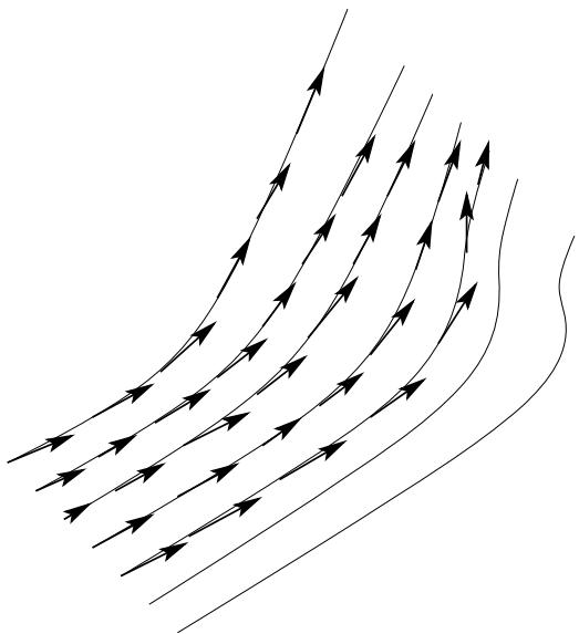
Figure 15.6 Streamlines representing the flow generated by a vector field

The curve ${\gamma }_p:\mathbb{R}\to M$ defined by ${\gamma }_p(t)={\sigma }_t(p)$ clearly passes through $p$ at $t=0$ . It is called the orbit of $p$ under the flow $\sigma$ and defines a tangent vector $X_p$ at $p$ by

$$X_{p}f=\frac{\mathrm{d}f({\gamma }_p(t))}{\mathrm{d}t}{|}_{t=0}=\frac{\mathrm{d}f({\sigma }_t(p))}{\mathrm{d}t}{|}_{t=0}.$$

Since $p$ is an arbitrary point of $M$ we have a vector field $X$ on $M,$ said to be the vector field induced by the flow $\sigma$. Any vector field $X$ induced by a one-parameter group of transformations of $M$ is said to be complete. The one-parameter group ${\sigma }_t$ can be though of as ‘filling in’ the vector field $X$ with a set of curves, which play the role of streamlines for a fluid whose velocity is everywhere given by $X$ (see Fig. 15.6).

Not every vector field is complete, but there is a local concept that is always applicable. A local one-parameter group of transformations, or local flow, consists of an open subset $U\subseteq M$ and a real interval $I_{ϵ}=(-ϵ,ϵ)$ , together with a map $\sigma :I_{ϵ}\times UM$ such that:

($i$ ) for each $t\in I_{ϵ}$ the map ${\sigma }_t:U\to M$ defined by ${\sigma }_t(p)=\sigma (t,p)$ ) is a diffeomorphism of $U$ onto ${\sigma }_t(U)$ ;

(ii ) if $t$, $s$ and $t+s\in I_{ϵ}$ and $p,{\sigma }_s(p)\in U$ then ${\sigma }_{t+s}(p)={\sigma }_t({\sigma }_s(p))$

A local flow induces a vector field $X$ on $U$ in a similar way to that described above for a flow:

$$X_{p}f=\frac{\mathrm{d}f({\sigma }_t(p))}{\mathrm{d}t}{|}_{t=0}\text{ for all }p\in U.\text{\hspace{1em}(15.28)}$$

It now turns out that every vector field $X$ corresponds to a local one-parameter group of transformations, which it may be said to generate.

Theorem 15.2 · Local flows of vector fields

If $X$ is a vector field on $M$, and $p\in M$ then there exists an interval $I=(-ϵ,ϵ)$ , a neighbourhood $U$ of $\dot{}p,$ , and a local flow $\sigma :I\times U\to M$ that induces the vector field $X{|}_U$ restricted to $U$.

Proof

If $(U,\varphi ;x^i)$ is a coordinate chart at $p$ we may set

$$X{|}_U=X^i\frac{\partial }{\partial x^i}\text{ where }{X}^i:U\to \mathbb{R}.$$

The existence and uniqueness theorem of ordinary differential equations implies that fo any $\mathbf{x}\in \varphi (U)$ there exists a unique curve $\mathbf{y}=\mathbf{y}(t;x^1,\dots ,x^n)$ ) on some interval $I=(-ϵ,ϵ)$ such that

$$\frac{\mathrm{d}{y}^i(t;x^1,\dots ,x^n)}{\mathrm{d}t}=X^i\circ {\varphi }^{-1}\left(y^1(t;\mathbf{x}),y^2(t;\mathbf{x}),\dots ,y^n(t;\mathbf{x})\right)$$

and

$$y^i(0;x^1,\dots ,x^n)=x^i.$$

As the solutions of a family of differential equations depend smoothly on the initial coordi nates [15, 16], the functions $y(t;x^1,\dots ,x^n)$ are differentiable with respect to $t$ and $x^i$

For fixed $s$ and fixed $\mathbf{x}\in \varphi (U)$ the curves $t\to z^i(t,s;\mathbf{x})=y^i(t;\mathbf{y}(s;\mathbf{x}))$ and $tz(t,s,\mathbf{x})=y^i(t+s;\mathbf{x})$ satisfy the same differential equation

$$\frac{\mathrm{d}{z}^i(t,s;x^1,\dots ,x^n)}{\mathrm{d}t}=X^i\left(z^1(t,s;\mathbf{x}),\dots ,z^n(t,s;\mathbf{x})\right)$$

and have the same initial conditions at $t=0.$

$$y^i(0;\mathbf{y}(s;\mathbf{x}))=y^i(s;\mathbf{x})=y^i(0+s;\mathbf{x}).$$

These solutions are therefore identical and the map $\sigma :I\times UU$ defined by $\sigma (t,p)={\varphi }^{-1}\mathbf{y}(t;\varphi (p))$ satisfies the local one-parameter group condition

$$\sigma (t,\sigma (s,p))=\sigma (t+s,p).$$

A useful consequence of this theorem is the local existence of a coordinate system that ‘straightens out’ any given vector field $X$ so that its components point along the 1-axis, $X^i=(1,0,\dots ,0)$ . The local flow ${\sigma }_t$ generated by $X$ is then simply a translation in the 1-direction, ${\sigma }_t(x^1,x^2,\dots ,x^n)=(x^1+t,x^2,\dots ,x^n)$

Theorem 15.3 · Local coordinate representation of a nonzero vector field

If $X$ is a vector field on a manifold $M$ such that $X_p\ne 0.$ , then there exists a coordinate chart $(U,\varphi ;x^i)$ at $p$ such that

$$X=\frac{\partial }{\partial x^1}.\text{\hspace{1em}(15.29)}$$

Proof outline

The idea behind the proof is not difficult. Pick any coordinate system $(U,\psi ;y^i)$ at $p$ such that $y^i(p)=0$ , and $X_p={\left({\partial }_{y^1}\right)}_p$ . Let $\sigma :I_{ϵ}\times A\to M$ be a local flow that induces $X$ on the open set $A.$ . In a neighbourhood of $p$ consider a small $(n-1)$ dimensional ‘open ball’ of points through $p$ that cuts across the flow, whose typical poin $q$ has coordinates $(0,y^2,\dots ,y^n)$ , and assign coordinates $(x^1=t,x^2=y^2,...,x^n=y^n)$

to points on the streamline ${\sigma }_t(q)$ through $q$. The coordinates $x^2,\dots ,x^n$ are then constan along the curves $t\to {\sigma }_t(q)$ , and the vector field $X,$ , being tangent to the streamlines, has coordinates $(1,0,\dots ,0)$ throughout a neighbourhood of $\dot{p}$ . A detailed proof may be found in [11, theorem 4.3] or [4, page 124]. -

Example 15.13

Let $X$ be the differentiable vector field $X=x^2{\partial }_x$ on the real line manifold $R$. To find a coordinate $y=y(x)$ ) such that $X={\partial }_{\nu }$ , we need to solve the differential equation

$$x^2\frac{\partial y}{\partial x}=1.$$

The solution is $y=C-1/x$

The local one-parameter group generated by $X$ is found by solving the ordinary differential equation,

$$\frac{\mathrm{d}x}{\mathrm{d}t}=x^2.$$

The solution is

$${\sigma }_t(x)=\frac{1}{x^{-1}-t}=\frac{x}{1-tx}.$$

It is straightforward to verify the group property

$${\sigma }_t({\sigma }_s(x))=\frac{x}{1-(t+s)x}={\sigma }_{t+s}(x).$$

Example 15.14

If $X$ and $Y$ are vector fields on $M$ generating flows ${\varphi }_t$ and ${\psi }_t$ respectively, let $\sigma$ be the curve through $p\in M$ defined by

$$\sigma (t)={\psi }_{-t}\circ {\varphi }_{-t}\circ {\psi }_t\circ {\varphi }_{t}p.$$

Then $\sigma (\sqrt{t})$ is a curve whose tangent vector is the commutator [$X$, $Y$] at $p$ . The proof is to let $f$ be any differentiable function at $p$ and show that

$$[X,Y{]}_{p}f=\underset{t\to 0}{\lim }\frac{f[\sigma (\sqrt{t})]-f[\sigma (0)]}{t}.$$

Details may be found in [3, $p$. 130]. Some interesting geometrophysical applications of this result are discussed in [17].

Lie derivative

Let $X$ be a smooth vector field on a manifold $M$, which generates a local one-parameter group of transformations ${\sigma }_t$ on $M$. If $Y$ is any differentiable vector field on $M$, we define its Lie derivative along $X$ to be

$${\mathcal{L}}_{X}Y=\underset{t\to 0}{\lim }\frac{Y-({\sigma }_t{)}_{\ast }Y}{t}.\text{\hspace{1em}(15.30)}$$

Figure 15.7 illustrates the siutation. Essentially, the tangent map of the diffeomorphism ${\sigma }_t$ is used to ‘drag’ the vector field $Y$ forward along the integral curves from a point ${\sigma }_{-t}(p)$ to $p$ and the result is compared with original value $Y_p$ of the vector field. Equation (15.7)

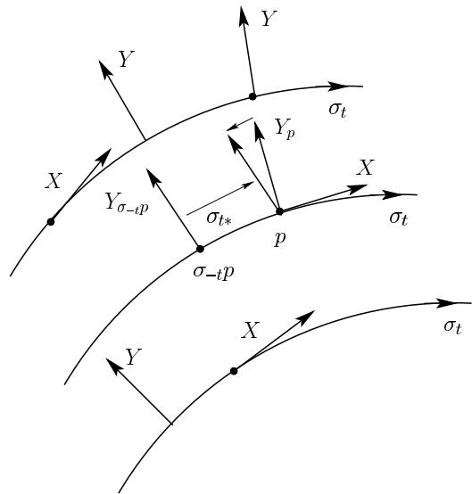
Figure 15.7 Lie derivative of a vector field $Y$ along a vector field $X$

performs this operation for neighbouring points and takes the limit on dividing by $t$. We now show that this derivative is identical with the ‘derivative-like’ operation of taking the commutator of two vector fields.

Let $f:M\to \mathbb{R}$ be a differentiable function, and $p$ any point of $M$. From Eq. (15.30) we have at $p$ ,

$$\begin{array}{l}({\mathcal{L}}_{X}Y{)}_{p}f={\lim }_{t\to 0}\frac{1}{t}(Y_{p}f-(({\sigma }_t{)}_{\ast }Y{)}_{p}f)\\ ={\lim }_{t\to 0}\frac{1}{t}(Y_{p}f-Y_{{\sigma }_{-t}(p)}(f\circ {\sigma }_t))\\ ={\lim }_{t\to 0}\frac{1}{t}(Y_{p}f-Y_{{\sigma }_{-t}(p)}f-Y_{{\sigma }_{-t}(p)}(f\circ {\sigma }_t-f))\\ ={\lim }_{t\to 0}\frac{1}{t}((Yf-(Yf)\circ {\sigma }_{-t})(p)-Y_{{\sigma }_{-t}(p)}(f\circ {\sigma }_t-f)).\end{array}$$

On setting $s=-t$ in the first term and using Eq. (15.28), the right-hand side reduces to $X(Yf)(p)-Y(Xf)(p)=[X,Y{]}_{p}f$ , and we have the desired relation

$${\mathcal{L}}_{X}Y=[X,Y].\text{\hspace{1em}(15.31)}$$

The concept of Lie derivative can be extended to all tensor fields. First, for any dif feomorphism $\phi :M\to M$ , we define the induced map $\tilde{\phi }:{\mathcal{T}}^{(r,s)}(M)\to {\mathcal{T}}^{(r,s)}(M)$ in the following way:

(i) for vector fields set $\tilde{\phi }={\phi }_{\ast }$ ;

(ii) for scalar fields $f:M\to$ $R$ set $\tilde{\phi }f=f\circ {\phi }^{-1}$ ;

(iii) for covector fields set $\tilde{\phi }={\left({\phi }^{-1}\right)}^{\ast }$

(iv) the map $\tilde{\phi }$ is extended to all tensor fields by demanding linearity and

$$\tilde{\phi }(T\otimes S)=\tilde{\phi }T\otimes \tilde{\phi }S$$

for arbitrary tensor fields $T$ and $S$.

If $\omega$ and $X$ are arbitrary covector and vector fields, then

$$⟨\tilde{\phi }\omega ,\tilde{\phi }X⟩=\tilde{\phi }⟨\omega ,X⟩,\text{\hspace{1em}(15.32)}$$

since

$$\begin{array}{r}⟨\tilde{\phi }\omega ,\tilde{\phi }X⟩(p)=⟨({\phi }^{-1}{)}^{\ast }{\omega }_{{\phi }^{-1}(p)},{\phi }_{\ast }{X}_{{\phi }^{-1}(p)}⟩\\ =⟨{\omega }_{{\phi }^{-1}(p)},X_{{\phi }^{-1}(p)}⟩=⟨\omega ,X⟩({\phi }^{-1}(p)).\end{array}$$

Exercise

For arbitrary vector fields $X$ show from (ii) that $\tilde{\phi }X(\tilde{\phi }f)=\tilde{\phi }(X(f))$

Using Eq. (15.11), property (iv) provides a unique definition for the application of the map $\tilde{\phi }$ to all higher order tensors. Alternatively, as for covector fields, the following is $a$ 4characterization of the map $\tilde{\phi };$

$$(\tilde{\phi }T)(\tilde{\phi }{\omega }^1,\dots ,\tilde{\phi }{\omega }^r,\tilde{\phi }{X}_1,\dots ,\tilde{\phi }{X}_s)=\tilde{\phi }(T({\omega }^1,\dots ,{\omega }^r,X_1,\dots ,X_s))$$

for all vector fields $X_1,\dots X_s$ and covector field ${\omega }^1,\dots ,{\omega }^r$

The Lie derivative ${\mathcal{L}}_{X}T$ of a smooth tensor field $T$ with respect to the vector field $X$ is defined as

$${\mathcal{L}}_{X}T=\underset{t\to 0}{\lim }\frac{1}{t}(T-{\tilde{\sigma }}_{t}T).\text{\hspace{1em}(15.33)}$$

Exercise

Show that for any tensor field $T$

$${\mathcal{L}}_{X}T=-\frac{\mathrm{d}{\tilde{\sigma }}_{t}T}{\mathrm{d}t}{|}_{t=0}\text{\hspace{1em}(15.34)}$$

and prove the Leibnitz rule

$${\mathcal{L}}_X(T\otimes S)=T\otimes ({\mathcal{L}}_{X}S)+({\mathcal{L}}_{X}T)\otimes S.\text{\hspace{1em}(15.35)}$$

When $T$ is a scalar field $f,$ , we find, on changing the limit variable to $s=-t$

$${\left({\mathcal{L}}_{X}f\right)}_p=\frac{\mathrm{d}f\circ {\sigma }_s(p)}{\mathrm{d}s}{|}_{s=0}=Xf(p),$$

and in a local coordinate chart $(U;x^i)$ )

$${\mathcal{L}}_{X}f=Xf=f_{,i}{X}^i.\text{\hspace{1em}(15.36)}$$

Since for any pair $i,j$

$${\mathcal{L}}_{{\partial }_{x^i}}\frac{\partial }{\partial x^j}=\left[\frac{\partial }{\partial x^i},\frac{\partial }{\partial x^j}\right]=\frac{{\partial }^2}{\partial x^i\partial x^j}-\frac{{\partial }^2}{\partial x^j\partial x^i}=0,$$

and ${\mathcal{L}}_{X}Y=[X,Y]=-[Y,X]=-{\mathcal{L}}_{Y}X$ for any pair of vector fields $X$, $Y$, we find

$${\mathcal{L}}_X\frac{\partial }{\partial x^j}=-{\mathcal{L}}_{{\partial }_{x^j}}\left(X^i\frac{\partial }{\partial x^i}\right)=-X_{,j}^i\frac{\partial }{\partial x^i}.$$

Applying the Leibnitz rule Eq. (15.35) results in

$${\mathcal{L}}_{X}Y={\mathcal{L}}_X\left(Y^i\frac{\partial }{\partial x^i}\right)=Y_{,j}^i{X}^j\frac{\partial }{\partial x^i}-Y^j{X}_{,j}^i\frac{\partial }{\partial x^i},$$

in agreement with the component formula for the Lie bracket in Eq. (15.25),

$${\left({\mathcal{L}}_{X}Y\right)}^i=Y_{,j}^i{X}^j-Y^j{X}_{,j}^i.\text{\hspace{1em}(15.37)}$$

To find the component formula for the Lie derivative of a 1-form $\omega =w_i\mathrm{d}{x}^i$ , we note that for any pair of vector fields $X$, $Y$

$${\mathcal{L}}_X⟨\omega ,Y⟩=X⟨\omega ,Y⟩=⟨{\mathcal{L}}_X\omega ,Y⟩+⟨\omega ,{\mathcal{L}}_{X}Y⟩,\text{\hspace{1em}(15.38)}$$

which follows from Eqs. Eq. (15.32) and Eq. (15.34),

$$\begin{array}{rl}& {\mathcal{L}}_X⟨\omega ,Y⟩=X⟨\omega ,Y⟩=-\frac{\mathrm{d}}{\mathrm{d}t}{\tilde{\sigma }}_t⟨\omega ,Y⟩{|}_{t=0}\\ & =-\frac{\mathrm{d}}{\mathrm{d}t}⟨{\tilde{\sigma }}_t\omega ,{\tilde{\sigma }}_{t}Y⟩{|}_{t=0}\\ & =-⟨\frac{\mathrm{d}}{\mathrm{d}t}{\tilde{\sigma }}_t\omega ,Y⟩{|}_{t=0}-⟨\omega ,\frac{\mathrm{d}}{\mathrm{d}t}{\tilde{\sigma }}_{t}Y⟩{|}_{t=0}\\ & =⟨{\mathcal{L}}_X\omega ,Y⟩+⟨\omega ,{\mathcal{L}}_{X}Y⟩.\end{array}$$

If $\omega =w_i\mathrm{d}{x}^i$ is a 1-form, then its Lie derivative ${\mathcal{L}}_X\omega$ with respect to the vector field $X$ has components in a coordinate chart $(U;x^i)$ given by

$$\begin{array}{rl}& {\left({\mathcal{L}}_X\omega \right)}_j=⟨{\mathcal{L}}_X\omega ,\frac{\partial }{\partial x^j}⟩\\ & ={\mathcal{L}}_X⟨\omega ,\frac{\partial }{\partial x^j}⟩-⟨\omega ,{\mathcal{L}}_X\frac{\partial }{\partial x^j}⟩\\ & ={\mathcal{L}}_X{w}_j+⟨\omega ,X_{,j}^i\frac{\partial }{\partial x^i}⟩\\ & =w_{j,i}{X}^i+w_i{X}_{,j}^i.\end{array}$$

Extending this argument to a general tensor of type ($r$, $s$), we find

$$\begin{array}{c}({\mathcal{L}}_{X}T{)}_{kl\dots }^{ij\dots }=T_{kl\dots ,m}^{ij\dots }{X}^m-T_{kl\dots }^{mj\dots }{X}_{,m}^i-T_{kl\dots }^{im\dots }{X}_{,m}^j-\dots \\ T_{ml\dots }^{ij\dots }{X}_{,k}^m+T_{km\dots }^{ij\dots }{X}_{,l}^m+\dots \end{array}\text{\hspace{1em}(15.39)}$$

Example 15.15

In local coordinates such that $X={\partial }_{x^1}$ (see Theorem 15.3), all $X^i{}_{,j}=0$ since the components $X^i=\mathrm{consts}$ . and the components of the Lie derivative are simply the derivatives in the 1-direction,

$${\left({\mathcal{L}}_{X}T\right)}_{kl\dots }^{ij\dots }=T_{kl\dots ,1}^{ij\dots }.$$

Problems

Problem 15.17

Show that the components ofthe Lie product $[X,Y{]}^k$ given by Eq. (15.25) transform as a contravariant vector field under a coordinate transformation $x^{\prime j}(x^i)$ ).

Problem 15.18

Show that the Jacobi identity can be written

$${\mathcal{L}}_{[X,Y]}Z={\mathcal{L}}_X{\mathcal{L}}_{Y}Z-{\mathcal{L}}_Y{\mathcal{L}}_{X}Z,$$

and this property extends to all tensors $T$ :

$${\mathcal{L}}_{[X,Y]}T={\mathcal{L}}_X{\mathcal{L}}_{Y}T-{\mathcal{L}}_Y{\mathcal{L}}_{X}T.$$

Problem 15.19

Let $\alpha :M\to N$ be a diffeomorphism between manifolds $M$ and $N$ and $X$ a vector field on $M$ that generates a local one-parameter group of transformations ${\sigma }_t$ on $M$. Show that the vector field $X^{\prime }={\alpha }_{\ast }X$ on $N$ generates the local flow ${\sigma }_t^{\prime }=\alpha \circ {\sigma }_t\circ {\alpha }^{-1}$

Problem 15.20

For any real positive number $n$ show that the vector field $X=x^n{\partial }_x$ is differentiable on the manifold ${\mathbb{R}}^{+}$ consisting ofthe positive real line $\{x\in \mathbb{R}\mid x>0\}$ . Why is this not true in genera on the entire real line $R$? As done for the case $n=2$ in Example 15.13, find the maximal one-paramete subgroup ${\sigma }_t$ generated by this vector field at any point $x>0$

Problem 15.21

On the manifold ${\mathbb{R}}^2$ with coordinates $(x,y)$ ), let $X$ be the vector field $X=-y{\partial }_x+x{\partial }_y$ . Determine the integral curve through any point $(x,y)$ , and the one-parameter group generated by $X$. Find coordinates $(x^{\prime },y^{\prime })$ such that $X={\partial }_{x^{\prime }}$

Problem 15.22

Repeat the previous problem for the vector fields, $X=y{\partial }_x+x{\partial }_y$ and $X=x{\partial }_x+y{\partial }_y$

Problem 15.23

On a compact manifold show that every vector field $X$ is complete. [Hint: Let ${\sigma }_t$ be a local flow generating $X,$ and let $ϵ$ be the least bound required on a finite open covering. Set ${\sigma }_t=({\sigma }_{t/N}{)}^N$ for $N$ large enough that $|t|<ϵN.]$

Problem 15.24

Show that the Lie derivative ${\mathcal{L}}_X$ commutes with all operations of contraction $C_j^i$ on a tensor field $T_{:}$

$${\mathcal{L}}_X{C}_j^{i}T=C_j^i{\mathcal{L}}_{X}T.$$

Problem 15.25

Prove the formula Eq. (15.39) for the Lie derivative of a general tensor.