16.5 Classical mechanics

中文

Classical analytic mechanics comes in two basic forms, Lagrangian or Hamiltonian. Both have natural formulations in the language of differential geometry, which we will outline in this section. More details may be found in [2, 10–14] and [4, chap. 13].

Calculus of variations

The reader should have at least a rudimentary acquaintance with the calculus of variations as found in standard texts on applied mathematics such as [15]. The following is a brief introduction to the subject, as it applies to parametrized curves on manifolds.

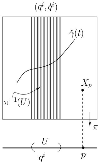
Figure 16.1 Tangent bundle

Let $M$ be any differential manifold and $TM$ its tangent bundle (refer to Section 15.3; see Fig. 16.1). If $\gamma :\mathbb{R}M$ is a smooth curve on $M$, define its lift to $TM$ to be the curve $\dot{\gamma }:\mathbb{R}\to TM$ traced out by the tangent vector to the curve, so tha $\dot{\gamma }(t)$ is the tangent vector to the curve at $\gamma (t)$ and $\pi (\dot{\gamma }(t))=\gamma (t)$

Exercise

Show that if $X(t)$ is the tangent to the curve $\dot{\gamma }(t)$ then ${\pi }_{\ast }X(t)=\dot{\gamma }(t)\in T_{\gamma (t)}(M)$

A function $L:TM\to \mathbb{R}$ is called a Lagrangian function, and for any parametrized curve $\gamma :[t_0,t_1]\to M$ we define the corresponding action to be

$$S[\gamma ]={\int }_{t_0}^{t_1}L(\dot{\gamma }(t))dt.\text{\hspace{1em}(16.21)}$$

If $(q^1,\dots ,q^n)$ are local coordinates on $M$ let the induced local coordinates on the tangent bundle $TM$ be written $(q^1,\dots ,q^n,{\dot{q}}^1,\dots ,{\dot{q}}^n)$ . This notation may cause a little concern to the reader, but it is much loved by physicists – the quantities ${\dot{\mathbf{q}}}^i$ are independent quantities, not to be thought of as ‘derivatives’ of $q^i$ unless a specific curve $\gamma$ having coordinate representation $q^i=q^i(t)$ is given. In that case, and only then, we find ${\dot{q}}^i(t)=\mathrm{d}{q}^i(t)/\mathrm{d}t$ along the $lift\dot{\gamma }(t)$ of the curve. Otherwise, the ${\dot{\mathbf{q}}}^i$ refer to all possible components oftangent vectors at that point of $M$ having coordinates $q^j.\mathrm{A}$ Lagrangian can be written as a function of 2$n$ variables, $L(q^1,\dots ,q^n,{\dot{q}}^1,\dots ,{\dot{q}}^n)$

By a variation ofa given curve $\gamma :[t_0,t_1]\to M$ (see Fig. 16.2) is meant a one-paramete family of curves $\gamma :[t_0,t_1]\times [-a,a]M$ such that for all $\lambda \in [-a,a]$

$$\gamma (t_0,\lambda )=\gamma (t_0)\text{ and }\gamma (t_1,\lambda )=\gamma (t_1)$$

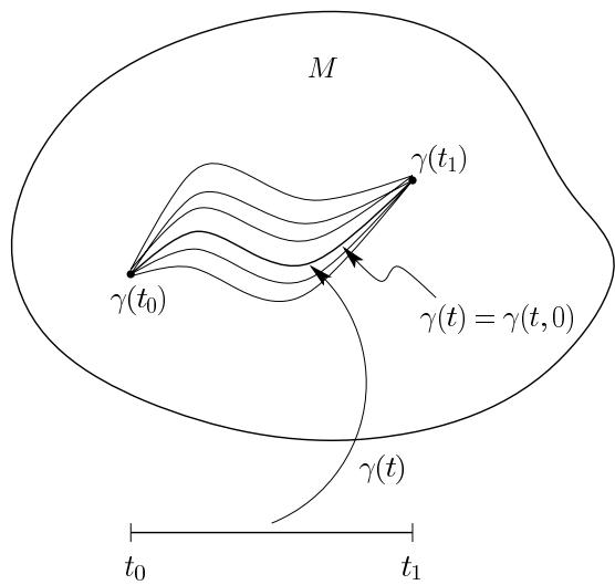
Figure 16.2 Variation of a curve

and the member of the family defined by $\lambda =0$ is the given curve $\gamma$ ,

$$\gamma (t,0)=\gamma (t)\text{ for all }{t}_0\le t\le t_1.$$

For each $t$ in the range $[t_0,t_1]$ we define the connection curve ${\gamma }_t:[-a,a]M$ by ${\gamma }_t(\lambda )=\gamma (t,\lambda )$ . Its tangent vector along the curve $\lambda =0$ is written $\delta \gamma$ , whose value at $t\in \left[t_0,t_1\right]$ is determined by the action on an arbitrary function $f:M\to \mathbb{R}$

$$\delta {\gamma }_t(f)=\frac{\partial f({\gamma }_t(\lambda ))}{\partial \lambda }{|}_{\lambda =0}.\text{\hspace{1em}(16.22)}$$

This is referred to as the variation field along the curve. In traditional literature it is simply referred to as the ‘variation of the curve’. Since all curves of the family meet at the end points $t=t_0,t_1$ , the quantity on the right-hand side of Eq. (16.22) vanishes,

$$\delta {\gamma }_{t_0}=\delta {\gamma }_{t_1}=0.\text{\hspace{1em}(16.23)}$$

The lift of the variation field to the tangent bundle is a curve $\delta \dot{\gamma }:[t_0,t_1]\to T{M}_{:}$ , which starts at the zero vector in the fibre above $\gamma (t_0)$ and ends at the zero vector in the fibre above $\gamma (t_1)$ . In coordinates.

$$\delta \dot{\gamma }(t)=\left(\delta q^1(t),\dots ,\delta q^n(t),\delta {\dot{q}}^1(t),\dots ,\delta {\dot{q}}^n(t)\right)$$

where

$$\delta q^i(t)={\frac{\partial q^i(t,\lambda )}{\partial \lambda }|}_{\lambda =0},\delta {\dot{q}}^i(t)={\frac{\partial {\dot{q}}^i(t,\lambda )}{\partial \lambda }|}_{\lambda =0}=\frac{\partial \delta q^i(t)}{\partial t}.$$

The action $S[\gamma ]$ becomes a function of $\lambda$ if $\gamma$ is replaced by its variation ${\gamma }_{\lambda }$ . We say that a curve $\gamma :[t_0,t_1]\to M$ is an extremal if for every variation of the curve

$$\delta S\equiv {\frac{\mathrm{d}S}{\mathrm{d}\lambda }|}_{\lambda =0}={\int }_{t_0}^{t_1}\delta L\mathrm{d}t=0\text{\hspace{1em}(16.24)}$$

where

$$\begin{array}{l}\delta L\equiv \frac{\partial L({\dot{\gamma }}_{\lambda })}{\partial \lambda }{|}_{\lambda =0}\\ =⟨\mathrm{d}L|\delta \dot{\gamma }⟩\\ =\frac{\partial L}{\partial q^i}\delta q^i+\frac{\partial L}{\partial {\dot{q}}^i}\delta {\dot{q}}^i.\end{array}$$

Substituting in Eq. (16.24) and performing an integration by parts results in

$$0=\delta S={\int }_{t_0}^{t_1}\left[\frac{\partial L}{\partial q^i}-\frac{\mathrm{d}}{\mathrm{d}t}\left(\frac{\partial L}{\partial {\dot{q}}^i}\right)\right]\mathrm{d}t+{\frac{\partial L}{\partial {\dot{q}}^i}\delta q^i|}_{t_0}^{t_1}.$$

The final term vanishes on account of $\delta q^i=0\mathrm{at}t=t_0,t_1$ , and since the $\delta q^i(t)$ are essentially arbitrary functions on the interval $[t_0,t_1]$ subject to the end-point constraints it may be shown that the term in the integrand must vanish,

$$\frac{\partial L}{\partial q^i}-\frac{\mathrm{d}}{\mathrm{d}t}\left(\frac{\partial L}{\partial {\dot{q}}^i}\right)=0.\text{\hspace{1em}(16.25)}$$

These are known as the Euler–Lagrange equations.

Example 16.5

In the plane, the shortest curve between two fixed points is a straight line. To prove this, use the length as action

$$S={\int }_{t_0}^{t_1}\sqrt{{\dot{x}}^2+{\dot{y}}^2}dt.$$

Setting $t=x$ and replacing˙ with there is a single variabl ${\mathbf{q}}^1=\mathbf{y}$ and the Lagrangian is $L=\sqrt{1+(y^{\prime }{)}^2}$ . The Euler–Lagrange equation reads

$$\frac{\partial L}{\partial x}-\frac{\mathrm{d}}{\mathrm{d}x}\left(\frac{\partial L}{\partial y^{\prime }}\right)=\frac{\mathrm{d}}{\mathrm{d}x}\left(\frac{y^{\prime }}{\sqrt{1+(y^{\prime }{)}^2}}\right)=0$$

with solution

$$\frac{y^{\prime }}{\sqrt{1+(y^{\prime }{)}^2}}=\text{ const. }$$

Hence $y^{\prime }=a$ for some constant ${}^{a,}$ , and the extremal curve is a straight line $y=ax+b$

Lagrangian mechanics

In Newtonian mechanics a dynamical system of $N$ particles is defined by positive rea scalars $m_1,m_2,...,m_N$ called the masses of the particles, and parametrized curves $t\mapsto {\mathbf{r}}_a={\mathbf{r}}_a(t)(a=1,2,...,N)$ where each ${\mathbf{r}}_a\in {\mathbb{R}}^3$ . The parameter $t$ is interpreted as time.

The kinetic energy of the system is defined as

$$T=\frac{1}{2}\sum _{a=1}^N{m}_a{\dot{\mathbf{r}}}_a^2\text{ where }{\dot{\mathbf{r}}}_a=\frac{\mathrm{d}{\mathbf{r}}_a}{\mathrm{d}t}\text{ and }{\dot{\mathbf{r}}}_a^2={\dot{x}}_a^2+{\dot{y}}_a^2+{\dot{z}}_a^2.$$

We will also assume conservative systems in which Newton’s second law reads

$$m_a{\ddot{\mathbf{r}}}_a=-{\nabla }_{a}U\equiv -\frac{\partial U({\mathbf{r}}_1,{\mathbf{r}}_2,\dots ,{\mathbf{r}}_N)}{\partial {\mathbf{r}}_a},\text{\hspace{1em}(16.26)}$$

where the given function $U:{\mathbb{R}}^{3N}\to r$ is known as the potential energy of the system.

A constrained system consists of a Newtonian dynamical system together with a manifold $M$ of dimension $n\le 3N$ , and a map $C:M\to {\mathbb{R}}^{3N}$ , called the constraint. In a local system of coordinates $(V;(q^1,q^2,\dots ,q^n))$ on $M$, the constraint can be written as a set of functions

$${\mathbf{r}}_a={\mathbf{r}}_a(q^1,q^2,\dots ,q^n)$$

and $n$ is called the number of degrees offreedom of the constrained system. The coordinates $q^i(i=1,\dots ,n)$ are commonly called generalized coordinates for the constrained system. They may be used even for an unconstrained system, in which $n=3N$ and $V$ is an open submanifold of ${\mathbb{R}}^{3N}$ ; in this case we are essentially expressing the original Newtonian dynamical system in terms of general coordinates. It will always be assumed that $(M,C)$ is an embedded submanifold of ${\mathbb{R}}^{3N}$ , so that the tangent map $C_{\ast }$ is injective everywhere. This implies that the matrix $[\partial {\mathbf{r}}_a/\partial q^i]$ has rank $n$ everywhere (no critical points).

Using the chain rule

$${\dot{\mathbf{r}}}_a=\frac{\partial {\mathbf{r}}_a}{\partial q^i}{\dot{q}}^i\text{ where }{\dot{q}}^i=\frac{\mathrm{d}{q}^i}{\mathrm{d}t}$$

the kinetic energy for a constrained system may be written

$$T=\frac{1}{2}{g}_{ij}{\dot{q}}^i{\dot{q}}^j\text{\hspace{1em}(16.27)}$$

where

$$g_{ij}=\sum _{a=1}^N{m}_a\frac{\partial {\mathbf{r}}_a}{\partial q^i}\cdot \frac{\partial {\mathbf{r}}_a}{\partial q^j}.\text{\hspace{1em}(16.28)}$$

This is a tensor field of type (0, 2) over the coordinate neighbourhood $V$, since

$$g_{i^{\prime }{j}^{\prime }}^{\prime }=\sum _{a=1}^N{m}_a\frac{\partial {\mathbf{r}}_a}{\partial q^{\prime i^{\prime }}}\cdot \frac{\partial {\mathbf{r}}_a}{\partial q^{\prime j^{\prime }}}=g_{ij}\frac{\partial q^i}{\partial q^{\prime i^{\prime }}}\frac{\partial q^j}{\partial q^{\prime j^{\prime }}}.$$

At each point of $q\in M$ we can define an inner product on the tangent space $T_q$

$$g(u,v)\equiv u\cdot v=g_{ij}{u}^i{v}^j\text{ where }u=u^i\frac{\partial }{\partial q^i},v=v^j\frac{\partial }{\partial q^j},$$

which is positive definite since

$$g(u,u)=\sum _{a=1}^N{m}_a{\left(\frac{\partial {\mathbf{r}}_a}{\partial q^i}{u}^i\right)}^2\ge 0$$

and the value 0 is only possible if ${\dot{u}}^i=0$ since the constraint map is an embedding and has no critical points. A manifold $M$ with a positive definite inner product defined everywhere is called a Riemannian manifold; further discussion of such manifolds will be found in Chapter 18. The associated symmetric tensor field $g=g_{ij}:\mathrm{d}{q}^i\otimes \mathrm{d}{q}^j$ is called the metric tensor. These remarks serve as motivation for the following definition.

A Lagrangian mechanical system consists of an $n$-dimensional Riemannian manifold $(M,g)$ called configuration space, together with a function $L:TM\to \mathbb{R}$ called the Lagrangian of the system. The Lagrangian will be assumed to have the form $L=T-U$ where, for any $u=(q^i,{\dot{q}}^j)\in TM$

$$T(u)=\frac{1}{2}g(u,u)=\frac{1}{2}{g}_{ij}(q^1,\dots ,q^n){\dot{q}}^i{\dot{q}}^j$$

and

$$U(u)=U(\pi (u))=U(q^1,\dots ,q^n).$$

As for the calculus of variations it will be common to write $L(q^1,\dots ,q^n,{\dot{q}}^1,\dots ,{\dot{q}}^n)$

The previous discussion shows that every constrained system can be considered as a Lagrangian mechanical system with $U(q^1,\dots ,q^n)=U({\mathbf{r}}_1(q^i),\dots ,{\mathbf{r}}_N(q^i))$ . In place of Newton’s law Eq. (16.26) we postulate Hamilton’s principle, that every motion $t\mapsto \gamma (t)\equiv q^i(t)$ of the system is an extremal of the action determined by the Lagrangian $L$

$$\delta S={\int }_{t_0}^{t_1}\delta L\mathrm{d}t=0.$$

The equations of motion are then the second-order differential equations Eq. (16.25),

$$\frac{\mathrm{d}}{\mathrm{d}t}\left(\frac{\partial L}{\partial {\dot{q}}^i}\right)-\frac{\partial L}{\partial q^i}=0,L=T-U\text{\hspace{1em}(16.29)}$$

known as Lagrange’s equations.

Example 16.6

A Newtonian system of $N$ unconstrained particles, ${\mathbf{r}}_a=(x_a,y_a,z_a)$ can be considered also as a Lagrangian system with $3N$ degrees of freedom if we set

$$q^1=x_1,q^2=y_1,q^3=z_1,q^4=x_2,\dots ,q^{3N}=z_N.$$

The metric tensor is diagonal with $g_{11}=m_1,g_{22}=m_1,...,g_{44}=m_2,...,$ , etc. Lagrange’s equations Eq. (16.29) read, for $i=3a-2(a=1,2,\dots ,N)$

$$\frac{\mathrm{d}}{\mathrm{d}t}\left(\frac{\partial L}{\partial {\dot{x}}_a}\right)-\frac{\partial L}{\partial x_a}=\frac{\mathrm{d}}{\mathrm{d}t}\left(m_a{\dot{x}}_a\right)+\frac{\partial U}{\partial x_a}=0,$$

that is,

$$m_a{\ddot{x}}_a=-\frac{\partial U}{\partial x_a}$$

and similarly

$$m_a{\ddot{y}}_a=-\frac{\partial U}{\partial y_a},m_a{\ddot{z}}_a=-\frac{\partial U}{\partial z_a}$$

in agreement with Eq. (16.26).

For a single particle, in spherical polar coordinates, $q^1=r>0,0<q^2=\theta <\pi ,0<q^3=\varphi <2\pi$

$$x=r\sin \theta \cos \varphi ,y=r\sin \theta \sin \varphi ,z=r\cos \theta$$

the kinetic energy is

$$T=\frac{m}{2}\left({\dot{x}}^2+{\dot{y}}^2+{\dot{z}}^2\right)=\frac{m}{2}\left({\dot{r}}^2+r^2{\dot{\theta }}^2+r^2{\sin }^2\theta {\dot{\varphi }}^2\right).$$

Hence the metric tensor $g$ has components

$$[g_{ij}]=\left(\begin{array}{ccc}m{\dot{r}}^2& 0& 0\\ 0& m{r}^2{\dot{\theta }}^2& 0\\ 0& 0& m{r}^2{\sin }^2\theta {\dot{\varphi }}^2\end{array}\right)$$

and Lagrange’s equations for a central potential $U=U(r)$ read

$$\begin{array}{c}m\ddot{r}-mr{\dot{\theta }}^2-mr{\sin }^2\theta {\dot{\varphi }}^2+\frac{\mathrm{d}U}{\mathrm{d}r}=0,\\ m\frac{\mathrm{d}}{\mathrm{d}t}(r^2\dot{\theta })-m{r}^2\sin \theta \cos \theta {\dot{\varphi }}^2=0,\\ m\frac{\mathrm{d}}{\mathrm{d}t}(r^2{\sin }^2\theta \dot{\varphi })=0.\end{array}$$

Exercise

Write out the equations of motion for a particle constrained to the plane $z=0$ in polar coordinates, $x=r\cos \theta ,y=r\sin \theta$

Example 16.7

The plane pendulum has configuration space $M=S^1$ , the one-dimensiona circle, which can be covered with two charts, $0<{\varphi }_1<2\pi$ and $-\pi <{\varphi }_2<\pi$ , such that on the overlaps they are related by

$$\begin{array}{l}{\theta }_2={\theta }_1\text{ for }0<{\theta }_1\le \pi \\ {\theta }_2={\theta }_1-2\pi \text{ for }\pi \le {\theta }_1<2\pi \end{array}$$

and constraint functions embedding this manifold in ${\mathbb{R}}^3$ are

$$\begin{array}{ll}x=0,& y=-a\sin {\theta }_1,z=-a\cos {\theta }_1;\\ x=0,& y=-a\sin {\theta }_2,z=-a\cos {\theta }_2.\end{array}$$

For $\theta ={\theta }_1$ or $\theta ={\theta }_2$ we have

$$T=\frac{m}{2}{a}^2{\dot{\theta }}^2,U=mgz=-mga\cos \theta ,L(\theta ,\dot{\theta })=T-U$$

and subsituting in Lagrange’s equations Eq. (16.29) with ${\mathbf{q}}^1=\mathbf{\theta }$ gives

$$\frac{\mathrm{d}}{\mathrm{d}t}\left(\frac{\partial L}{\partial \dot{\theta }}\right)-\frac{\partial L}{\partial \theta }=m{a}^2\ddot{\theta }+mga\sin \theta =0.$$

For small values of $\nabla \cdot {\theta }_{:}$ , the pendulum hanging near vertical, the equation approximates the simple harmonic oscillator equation

$$\ddot{\theta }+\frac{g}{a}\theta =0$$

with period $\tau =2\pi \sqrt{g/a}$

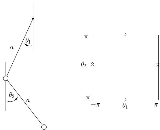
Figure 16.3 Double pendulum

Example 16.8

The spherical pendulum is similar to the plane pendulum, but the config uration manifold is the 2-sphere $S^2$ . In spherical polars the constraint is

$$x=a\sin \theta \cos \varphi ,y=a\sin \theta \sin \varphi ,z=-a\cos \theta$$

and as for Example 16.6 we find

$$T=\frac{m}{2}{a}^2({\dot{\theta }}^2+{\sin }^2\theta {\dot{\varphi }}^2),U=mgz=-mga\cos \theta .$$

Exercise

Write out Lagrange’s equations for the spherical pendulum

Example 16.9

The double pendulum consists of two plane pendula, of lengths $a$, $b$ and equal mass $m$, one suspended from the end of the other (see Fig. 16.3). The configuration manifold is the 2-torus $M=S^1\times S^1=T^2$ , and constraint functions are

$$x_1=x_2=0,y_1=-a\sin {\theta }_1,z_1=-a\cos {\theta }_1,$$ $$y_2=-a\sin {\theta }_1-b\sin {\theta }_2,z_2=-a\cos {\theta }_1-b\cos {\theta }_2.$$

The kinetic energy is

$$\begin{array}{l}T=\frac{m}{2}\left({\dot{y}}_1^2+{\dot{z}}_1^2+{\dot{y}}_2^2+{\dot{z}}_2^2\right)\\ =\frac{m}{2}\left(2a^2{\dot{\theta }}_1^2+b^2{\dot{\theta }}_2^2+2ab\cos ({\theta }_1-\theta -2){\dot{\theta }}_1{\dot{\theta }}_2\right)\end{array}$$

and the potential energy is $U=-2mga$ $\cos$ ${\theta }_1-mgb$ $\cos$ ${\theta }_2$.

Exercise

Write out Lagrange’s equations for the double pendulum of this example

Exercise

Write out the Lagrangian for a double pendulum with unequal masses, $m_1$ and $m_2$ .

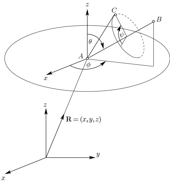
Figure 16.4 Degrees of freedom of a rigid body

Example 16.10

A rigid body is a system of particles subject to the constraint that al distances between particles are constant, $|{\mathbf{r}}_a-{\mathbf{r}}_b|=c_{ab}=\mathrm{const}$ . These equations are no independent since their number is considerably greater in general than the number of components in the ${\mathbf{r}}_a$ . The number of degrees of freedom is in general six, as can be seen from the following argument. Fix a point in the object $A$, such as its centre of mass, and assign to it three rectangular coordinates $\mathbf{R}=(X,Y,Z)$ . Any other point $B$ of the body is at a fixed distance from $A$ and therefore is constrained to move on a sphere about $A$. It can be assigned two spherical angles $\theta$, $\varphi$ as for the spherical pendulum. The only remaining freedom is a rotation by an angle $\psi$ , say, about the axis $AB$. Every point of the rigid body is now determined once these three angles are specified (see Fig. 16.4). Thus the configuration manifold of the rigid body is the six-dimensional manifold ${\mathbb{R}}^3\times S^2\times S^1$ . Alternatively the freedom of the body about the point $A$ may be determined by a member of the rotation group $SO(3)$ , which can be specified by three Euler angles. These are the most commonly used generalized coordinates for a rigid body. Details may be found in [12, chap. 6].

Given a tangent vector $u=\dot{\gamma }={\dot{q}}^i{\partial }_{q^i}$ , the momentum 1-form conjugate to $u$ is defined by

$$⟨{\omega }_u,v⟩=g(u,v)=g_{ij}{\dot{q}}^i{v}^j.$$

Setting ${\omega }_u=p_i\mathrm{d}{q}^i$ we see that

$$p_i=g_{ij}{\dot{q}}^j=\frac{\partial L}{\partial {\dot{q}}^i}.\text{\hspace{1em}(16.30)}$$

The last step follows either by direct differentiation of $L=\frac{1}{2}{g}_{ij}{\dot{q}}^i{\dot{q}}^j-U(q)$ or by applying Euler’s theorem on homogeneous functions to $T(q^j,\lambda {\dot{q}}^i)={\lambda }^{2}T(q^j,{\dot{q}}^i)$ ). The components $p_i$ of the momentum 1-form, given by Eq. (16.30), are called the generalized momenta conjugate to the generalized coordinates $q^i$

Exercise

For a general Lagrangian $L$, not necessarily of the form $T-U,$ , show that $\omega =(\partial L/\partial {\dot{q}}^i)\mathrm{d}{q}^i$ is a well-defined 1-form on $M$.

Example 16.11

The generalized momentum for an unconstrained particle $\begin{array}{r}L=\frac{1}{2}m{\dot{\mathbf{r}}}^2-\end{array}U(\mathbf{r})$ given by

$$p_x=\frac{\partial L}{\partial \dot{x}}=m\dot{x},p_y=\frac{\partial L}{\partial \dot{y}}=m\dot{y},p_z=\frac{\partial L}{\partial \dot{z}}=m\dot{z},$$

which are the components of standard momentum $\mathbf{p}=(p_x,p_y,p_z)=m\dot{\mathbf{r}}.$

In spherical polar coordinates

$$L=\frac{m}{2}({\dot{r}}^2+r^2{\dot{\theta }}^2+r^2{\sin }^2\theta {\dot{\varphi }}^2)-U(r,\theta ,\varphi ),$$

whence

$$p_{\varphi }=\frac{\partial L}{\partial \dot{\varphi }}=m{r}^2\dot{\varphi }{\sin }^2\theta .$$

This can be identified with the $z$-component of angular momentum,

$$L_z=\mathbf{r}\times \mathbf{p}\cdot \hat{\mathbf{z}}=m(x\dot{y}-y\dot{x})=m\dot{\varphi }{r}^2{\sin }^2\theta .$$

It is a general result that the momentum conjugate to an angular coordinate about a fixed axis is the angular momentum about that axis.

Exercise

The angle $\theta$ in the previous example does not have a fixed axis ofdefinition unless $\varphi =\mathrm{const}.$ In this case show that $p_{\theta }=\mathbf{L}\cdot (-\cos \varphi ,\sin \varphi ,0)$ and interpret geometrically.

Example 16.12

If the Lagrangian has no explicit dependence on a particular generalized coordinate $q^k$ , so that $\partial L/\partial q^k=0$ , it is called an ignorable or cyclic coordinate, The corresponding generalized momentum $p_k$ is then a constant of the motion, for the $k$th Lagrange’s equation reads

$$0=\frac{\mathrm{d}}{\mathrm{d}t}\frac{\partial L}{\partial {\dot{q}}^k}-\frac{\partial L}{\partial q_k}=\frac{\mathrm{d}{p}_k}{\mathrm{d}t}.$$

This is a particular instance of a more general statement, known as Noether’s theorem.

Let ${\phi }_s:M\to M$ be a local one-parameter group of motions on $M$, generating the vecto field $X$ by

$$X_{q}f=\frac{\partial f({\phi }_s(q))}{\partial s}{|}_{s=0}.$$

The tangent map ${\phi }_{\ast s}$ induces a local flow on the tangent bundle, since ${\phi }_{\ast s}\circ {\phi }_{\ast t}=({\phi }_s{\phi }_t{)}_{\ast }={\phi }_{\ast (s+t)}$ , and the Lagrangian is said to be invariant under this local one-parameter group if $L({\phi }_{\ast s}u)=L(u)$ for all $u\in TM$ . Noether’s theorem asserts that the quantity $⟨{\omega }_u,X⟩$ is then a constant of the motion. The result is most easily proved in natural coordinates on $TM$

Let $q^i(t)$ be any solution of Lagrange’s equations, and set $\mathbf{q}(s,t)={\phi }_s\mathbf{q}(t)$ . On differentiation with respect to $t$ we have

$$\dot{\mathbf{q}}(s,t)={\phi }_s\dot{\mathbf{q}}(t)=\frac{\partial \mathbf{q}(s,t)}{\partial t}$$

and invariance of the Lagrangian implies, using Lagrange’s equations at $s=0$

$$\begin{array}{l}0=\frac{\partial L}{\partial s}{|}_{s=0}=\frac{\partial }{\partial s}(L(\mathbf{q}(s,t),\dot{\mathbf{q}}(s,t))){|}_{s=0}\\ =(\frac{\partial L}{\partial q^i}\frac{\partial q^i}{\partial s}+\frac{\partial L}{\partial {\dot{q}}^i}\frac{\partial {\dot{q}}^i}{\partial s}){|}_{s=0}\\ =\left(\frac{\partial }{\partial t}\right(\frac{\partial L}{\partial {\dot{q}}^i})\frac{\partial q^i}{\partial s}+\frac{\partial L}{\partial {\dot{q}}^i}\frac{{\partial }^2{q}^i}{\partial s\partial t}){|}_{s=0}\\ =\frac{\partial }{\partial t}\left(\frac{\partial L}{\partial {\dot{q}}^i}\frac{\partial q^i}{\partial s}\right){|}_{s=0}\\ =\frac{\partial }{\partial t}(p_i{X}^i).\end{array}$$

Hence, along any solution of Lagrange’s equations, we have an integral of the motion

$$⟨{\omega }_u,X⟩=g_{ij}{\dot{q}}^i{X}^j=p_i{X}^j=\text{ const }.$$

The one-parameter group is often called a symmetry group of the system, and Noether’s theorem exhibits the relation between symmetries and conservation laws.

If $q^k$ is an ignorable coordinate then the one-parameter group of motions

$${\phi }_s(\mathbf{q})=(q^1,\dots ,q^{k-1},q^k+s,q^{k+1},\dots ,q^n)$$

is an invariance group of the Lagrangian. It generates the vector field $X^i=\partial ({\phi }_s(\mathbf{q}){)}^i/\partial s{|}_{s=0}={\delta }_k^i$ , and the associated constant of the motion is the generalized momentum $p_i{X}^i=p_i{\delta }_k^i=p_k$ conjugate to the ignorable coordinate.

Hamiltonian mechanics

A 2-form $\Omega$ is said to be non-degenerate at $p\in M$ if

$${\Omega }_p(X_p,Y_p)=0\text{ for all }{Y}_p\in T_p(M)⟹X_p=0.$$

As for the concept of non-singularity for inner products (Chapter 5), this is true if and only $\mathrm{if}$

$${\Omega }_p=A_{ij}{\left(\mathrm{d}{x}^i\right)}_p\wedge {\left(\mathrm{d}{x}^j\right)}_p\text{ where }{A}_{ij}=-A_{ji},\det [A_{ij}]\ne 0.$$

Exercise

Prove this statement.

The manifold $M$ must necessarily be of even dimension $m=2n$ if there exists a non degenerate 2-form, since $\det A\det {\mathbf{A}}^T=\det (-\mathbf{A})=(-1{)}^m\det A$. A symplectic structure on a $2n$-dimensional manifold $M$ is a closed differentiable 2-form $\Omega$ that is everywhere non-degenerate. Recall that closed means that $\mathrm{d}\Omega =0$ everywhere. An even-dimensiona manifold $M$ with a symplectic structure is called a symplectic manifold.

As in Examples 7.6 and 7.7, a symplectic form $\Omega$ induces an isomorphic map $\bar{\Omega }$ : $T_p(M)\to T_p^{\ast }(M)$ where the covector $\overline{{\mathbf{X}}_{\mathbf{p}}}=\bar{\Omega }{\mathbf{X}}_{\mathbf{p}}$ is defined by

$$⟨\overline{X_p},Y_p⟩\equiv ⟨\bar{\Omega }{X}_p,Y_p⟩=\Omega (X_p,Y_p).\text{\hspace{1em}(16.31)}$$

We may naturally extend this correspondence to one between vector fields and differentia 1-forms $X\overline{X}$ such that for any vector field $Y$

$$⟨\overline{X},Y⟩=\Omega (X,Y).$$

By $Eq.$ Eq. (16.10), we find for any vector field

$$\overline{X}=\frac{1}{2}{\mathrm{i}}_X\Omega .\text{\hspace{1em}(16.32)}$$

In components ${\overline{X}}_i=A_{ji}{X}^j$

We will write the vector field corresponding to a 1-form by the same notation $\overline{\omega }={\bar{\Omega }}^{-1}\omega$ , such that

$$⟨\omega ,Y⟩=\Omega (\overline{\omega },Y)\text{\hspace{1em}(16.33)}$$

for all vector fields $Y$. A vector field $X$ is said to be a Hamiltonian vector field if there exists a function $H$ on $M$ such that $X=\overline{\mathrm{d}H}$ , or equivalently $\overline{X}=\mathrm{d}H$ . The function $H$ is called the Hamiltonian generating this vector field. A function $f$ is said to be a first integral of the phase flow generated by the Hamiltonian vector field $X=\overline{\mathrm{d}H}\mathrm{if}Xf=0$ The Hamiltonian $H$ is a first integral of the phase flow, for

$$X(H)=⟨\mathrm{d}H,X⟩=⟨\mathrm{d}H,\overline{\mathrm{d}H}⟩=\Omega (\overline{\mathrm{d}H},\overline{\mathrm{d}H})=0$$

on setting $\omega =\mathrm{d}H$ and $Y=\overline{\mathrm{d}H}$ in Eq. (16.33) and using the antisymmetry of $\Omega$.

Any function $f:M\to R$ is known as a dynamical variable. For any dynamical variable $f$ we set $X_f=\overline{\mathrm{d}}\overline{f}$ to be the Hamiltonian vector field generated by $f.$ . Then for any vector field $Y$,

$$\Omega (X_f,Y)=⟨\overline{X_f},Y⟩=⟨\mathrm{d}f,Y⟩=Y(f),$$

and we have the identity

$${\mathrm{i}}_{X_f}\Omega =2\mathrm{d}f.$$

Define the Poisson bracket of two dynamical variables $f$ and $g$ to be

$$(f,g)=\Omega (X_f,X_g),\text{\hspace{1em}(16.34)}$$

from which

$$(f,g)=⟨\mathrm{d}f,X_g⟩=X_{g}f=-X_{f}g=-(f,g).$$

In these and other conventions, different authors adopt almost random sign conventions – so beware of any discrepencies between formulae given here and those in other books!

From Eq. (16.13) we have that $\mathrm{d}\Omega =0$ implies

$${\mathcal{L}}_X\Omega ={\mathrm{i}}_X\mathrm{d}\Omega +\mathrm{d}\circ {\mathrm{i}}_X\Omega =\mathrm{d}({\mathrm{i}}_X\Omega ),$$

whence the Lie derivative of the symplectic form in any Hamiltonian direction vanishes,

$${\mathcal{L}}_{X_f}\Omega =2\mathrm{d}(\mathrm{d}f)=2{\mathrm{d}}^{2}f=0.$$

Using Eq. (16.12) with $X=X_f$ and $Y=Y_g$ we obtain

$${\mathrm{i}}_{[X_f,X_g]}\Omega ={\mathcal{L}}_{X_f}\left({\mathrm{i}}_{X_g}\Omega \right).$$

By Eq. (16.8),

$${\mathrm{i}}_{[X_f,X_g]}\Omega =2{\mathcal{L}}_{X_f}\mathrm{d}g=2\mathrm{d}{\mathcal{L}}_{X_f}g=2\mathrm{d}(X_{f}g)={\mathrm{i}}_{X_{(g,f)}}\Omega ,$$

whence

$$[X_f,X_g]=X_{(g,f)}=-X_{(f,g)}.\text{\hspace{1em}(16.35)}$$

From the Jacobi identity (15.24) it then follows that

$$((f,g),h)+((g,h),f)+((h,f),g)=0.\text{\hspace{1em}(16.36)}$$

Exercise

Prove Eq. (16.36).

Exercise

Show that $(f,g)+(f,h)=(f,g+h)\mathrm{and}(f,gh)=g(f,h)+h(f,g).$

The rate of change of a dynamical variable $f$ along a Hamiltonian flow is given by

$$\dot{f}=\frac{\mathrm{d}f}{\mathrm{d}t}=X_{H}f=(f,H).\text{\hspace{1em}(16.37)}$$

Thus $f$ is a first integral of the phase flow generated by the Hamiltonian vector field $X_H$ if and only if it commutes’ with the Hamiltonian, in the sense that its Poisson bracket with $H$ vanishes, $(f,H)=0$ . The analogies with quantum mechanics (Chapter 14) are manifest.

Exercise

Show that if $f$ and $g$ are first integrals then so is $(f,g)$

Example 16.13

Let $M={\mathbb{R}}^{2n}$ with coordinates labelled $(q^1,\dots ,q^n,p_1,\dots ,p_n)$ . The 2- form $\Omega =2\mathrm{d}{q}^i\wedge \mathrm{d}{p}_i=\mathrm{d}{q}^i\otimes \mathrm{d}{p}_i-\mathrm{d}{p}_i\otimes \mathrm{d}{q}^i$ , having constant components

$$\mathsf{A}=\left(\begin{array}{cc}\mathsf{O}& \mathsf{I}\\ -\mathsf{I}& \mathsf{O}\end{array}\right)$$

is a symplectic structure, since $\det \mathsf{A}=1$ (a simple exercise!) and it is closed,

$$\mathrm{d}\Omega =2{\mathrm{d}}^2{q}^i\wedge \mathrm{d}{p}_i-\mathrm{d}{q}^i\wedge {\mathrm{d}}^2{p}_i=0.$$

If $X$ and $Y$ are vector fields having components

$$X={\xi }^i\frac{\partial }{\partial q^i}+{\xi }_j\frac{\partial }{\partial p_j},Y={\eta }^i\frac{\partial }{\partial q^i}+{\eta }_j\frac{\partial }{\partial p_j},$$

then

$$⟨\overline{X},Y⟩=\Omega (X,Y)=(\mathrm{d}{q}^i\otimes \mathrm{d}{p}_i-\mathrm{d}{p}_i\otimes \mathrm{d}{q}^i)(X,Y)={\xi }^i{\eta }_i-{\xi }_i{\eta }^i$$

so that the 1-form $\overline{\mathbf{X}}$ has components

$$\overline{X}=-{\xi }_j\mathrm{d}{q}^j+{\xi }^i\mathrm{d}{p}_i.$$

A Hamiltonian vector field $X$ has ${\xi }_j=-\partial H/\partial q^i$ and ${\xi }^i=\partial H/\partial p_i$ , so that

$$X=\overline{\mathrm{d}H}=X_H=\frac{\partial H}{\partial p_i}\frac{\partial }{\partial q^i}-\frac{\partial H}{\partial q^j}\frac{\partial }{\partial p_j}.$$

A curve $\gamma :\mathbb{R}M$ is an integral curve of this vector field if the functions $q^i=q^i(t)p_j=p_j(t)$ satisfy the differential equations known as Hamilton’s equations:

$$\frac{\mathrm{d}{q}^i}{\mathrm{d}t}=\frac{\partial H}{\partial p_i},\frac{\mathrm{d}{p}_j}{\mathrm{d}t}=-\frac{\partial H}{\partial q^j}.\text{\hspace{1em}(16.38)}$$

The Poisson bracket is given by

$$(f,g)=X_{g}f=(\frac{\partial g}{\partial p_i}\frac{\partial }{\partial q^i}-\frac{\partial g}{\partial q^j}\frac{\partial }{\partial p_j})f=\frac{\partial f}{\partial q^i}\frac{\partial g}{\partial p_i}-\frac{\partial f}{\partial p_j}\frac{\partial g}{\partial q^j}.$$

For any dynamical variable $f$ it is straightforward to verify the Poisson bracket relations

$$(q^i,f)=\frac{\partial f}{\partial p_i},(p_i,f)=-\frac{\partial f}{\partial q^i},\text{\hspace{1em}(16.39)}$$

from which the canonical relations are immediate

$$(q^i,q^j)=0,(p_i,p_j)=0,(q^i,p_j)={\delta }_j^i.$$

Connection between Lagrangian and Hamiltonian mechanics

If $M$ is a manifold ofany dimension $n$ its cotangent bundle $T^{\ast }{M}_{:}$ , consisting of all covectors at all points, is a $2n$-dimensional manifold. If $(U;q^i)$ is any coordinate chart on $M,$ a chart is generated on $T^{\ast }M$ by assigning coordinates $(q^1,\dots ,q^n,p_1,\dots ,p_n)$ to any covector ${\omega }_q=p_i(\mathrm{d}{q}^i{)}_q$ at $q\in M$ . The natural projection map $\pi :T^{\ast }M\to M$ has the effect of sending any covector to its base point, $\pi ({\omega }_q)=q$ . The tangent map corresponding to this projection map, ${\pi }_{\ast }:T_{{\omega }_q}(T^{\ast }M)\to T_q(M)$ , maps every tangent vector $X_{{\omega }_q}\in T_{{\omega }_q}(T^{\ast }M)$ to a tangent vector ${\pi }_{\ast }{X}_{{\omega }_q}\in T_q(M)$ . In canonical coordinates, set

$$X_{{\omega }_q}={\xi }^i\frac{\partial }{\partial q^i}+{\xi }_j\frac{\partial }{\partial p_j}$$

and for any function $f:M\to \mathbb{R}$ , written in coordinates as $f(q^1,\dots ,q^n)$ , we have

$$\left({\pi }_{\ast }{X}_{{\omega }_q}\right)f(\mathbf{q})=X_{{\omega }_q}\left(f\circ \pi \right)(\mathbf{q},\mathbf{p})={\xi }^i\frac{\partial f(\mathbf{q})}{\partial q^i}+{\xi }_i\frac{\partial f(\mathbf{q})}{\partial p_i}$$

so that

$${\pi }_{\ast }{X}_{{\omega }_q}={\xi }^i\frac{\partial }{\partial q^i}.$$

This defines a canonical 1-form $\theta$ on $T^{\ast }M$ by setting

$${\theta }_{{\omega }_q}(X_{{\omega }_q})\equiv ⟨{\theta }_{{\omega }_q},X_{{\omega }_q}⟩=⟨{\omega }_q,{\pi }_{\ast }{X}_{{\omega }_q}⟩.$$

Alternatively, we can think of $\theta$ as the pullback ${\theta }_{{\omega }_q}={\pi }^{\ast }{\omega }_q\in T{\ast }_{{\omega }_q}(T^{\ast }M)$ , for

$$⟨{\pi }^{\ast }{\omega }_q,X_{{\omega }_q}⟩=⟨{\omega }_q,{\pi }_{\ast }{X}_{{\omega }_q}⟩={\theta }_{{\omega }_q}(X_{{\omega }_q})$$

for arbitrary $X_{{\omega }_q}\in T_{{\omega }_q}(T^{\ast }M)$ . Writing ${\omega }_q=p_i\mathrm{d}{q}^i$ , we thus have $⟨{\theta }_{{\omega }_q},X_{{\omega }_q}⟩=p_i{\xi }^i$ , so that in any canonical chart $(U\times {\mathbb{R}}^n;q^1,\dots ,q^n,p_1,\dots ,p_n)$

$$\theta =p_i\mathrm{d}{q}^i.\text{\hspace{1em}(16.40)}$$

The 2-form

$$\Omega =-2\mathrm{d}\theta =2\mathrm{d}{q}^i\wedge \mathrm{d}{p}_i\text{\hspace{1em}(16.41)}$$

is of the same form as that in Example 16.13, and provides a natural symplectic structure on the cotangent bundle of any manifold $M$.

Given a Lagrangian system having configuration space ($M$, $g$) and Lagrangian function $L=T-U:TM\to \mathbb{R}$ where

$$T(\mathbf{q},\dot{\mathbf{q}})=\frac{1}{2}{g}_{ij}(\mathbf{q}){\dot{q}}^i{\dot{q}}^j,U=U(\mathbf{q})$$

the cotangent bundle $T^{\ast }M$ , consisting of momentum 1-forms on $M$, is known as the phase space of the system. The coordinates $p_i$ and ${\dot{q}}^j$ are related by Eq. (16.30), so that velocity components can be expressed in terms ofgeneralized momenta, ${\dot{q}}^j=g^{jk}{p}_k$ where $g^{jk}{g}_{ki}={\delta }_{i:}^j$ , and Lagrange’s equations Eq. (16.29) can be written

$${\dot{p}}_i=\frac{\partial L}{\partial q^i}.$$

Our first task is to find a Hamiltonian function $H:T^{\ast }M\to \mathbb{R}$ , written $H(q^1,\dots ,q^n{p}_1,\dots ,p_n)$ , such that the equations of motion of the system in phase space have the form of Hamiltonian equations Eq. (16.38) in Example 16.13. The Hamiltonian function $H$ mus then have exterior derivative

$$\begin{array}{l}\mathrm{d}H=\frac{\partial H}{\partial q^i}\mathrm{d}{q}^i+H{p}_i\mathrm{d}{p}_i\\ =-{\dot{p}}_i\mathrm{d}{q}^i+{\dot{q}}^i\mathrm{d}{p}_i\\ =-\frac{\partial L}{\partial q^i}\mathrm{d}{q}^i+\mathrm{d}({\dot{q}}^i{p}_i)-p_i\mathrm{d}{\dot{q}}^i\\ =\mathrm{d}({\dot{q}}^i{p}_i)-\left(\frac{\partial L}{\partial q^i}\mathrm{d}{q}^i+\frac{\partial L}{\partial {\dot{q}}^j}\mathrm{d}{\dot{q}}^j\right)\\ =\mathrm{d}({\dot{q}}^i{p}_i-L)\end{array}$$

whence, within an arbitrary constant

$$H={\dot{q}}^i{p}_i-L=g_{ij}{\dot{q}}^i{\dot{q}}^j-L=2T-(T-U)=T+U=E.$$

The Hamiltonian is thus the energy of the system expressed in terms ofcanonical coordinates on $T^{\ast }M$

Apart from expressing the equations of mechanics as a first-order system of equations, one of the advantages of the Hamiltonian view is that coordinates in which the symplectic form takes the form given in Example 16.13 need not be restricted to the canonical coordi nates generated by the tangent bundle construction. For example, let $(q^i,p_j)({\bar{q}}^i,{\bar{p}}_j)$ ) be any coordinate transformation such that the canonical 1-forms $\theta =p_i$ $\mathrm{d}{q}^i$ and $\bar{\theta }={\bar{p}}_i\mathrm{d}{\bar{q}}^i$ generate the same symplectic form,

$$\bar{\Omega }=-2\mathrm{d}\bar{\theta }=\Omega =-2\mathrm{d}\theta$$

so that $\bar{\theta }=\theta -\mathrm{d}F$ for some function $F$ on $T^{\ast }M$

Exercise

Show that ${\bar{p}}_i\frac{\partial {\bar{q}}^i}{\partial p_j}=-\frac{\partial F}{\partial p_j},{\bar{p}}_i\frac{\partial {\bar{q}}^i}{\partial q^j}=p_j-\frac{\partial F}{\partial q^j}.$

Since $\Omega =\bar{\Omega }$ the Hamiltonian vector fields generated by any dynamical variable $f,$ are identical for the two forms, $X_f={\bar{X}}_f$ , since for any vector field $Y$ on $T^{\ast }M$

$$\bar{\Omega }({\bar{X}}_f,Y)=Yf=\Omega (X_f,Y).$$

Hence, Poisson brackets are invariant with respect to this change of coordinates, for

$$(f,g{)}_{\bar{q},\bar{p}}={\bar{X}}_{g}f=X_{g}f=(f,g{)}_{g,p}.$$

This result is easy to prove directly by change of variables, as is done in some standard books on analytic mechanics. Using Eqs. Eq. (16.37) and Eq. (16.39) we have then

$$\frac{\mathrm{d}{\bar{q}}^i}{\mathrm{d}t}=({\bar{q}}^i,H{)}_{q,p}=({\bar{q}}^i,H{)}_{\bar{q},\bar{p}}=\frac{\partial H}{\partial {\bar{p}}_i},$$ $$\frac{\mathrm{d}{\bar{p}}_i}{\mathrm{d}t}=({\bar{p}}_i,H{)}_{q,p}=({\bar{p}}_i,H{)}_{\bar{q},\bar{p}}=-\frac{\partial H}{\partial {\bar{q}}^i},$$

and Hamilton’s equations are preserved under such transformations. These are called homogeneous contact transformations.

More generally, let $H(q^1,\dots ,q^n,p_1,\dots ,p_n,t)$ be a time-dependent Hamiltonian, de fined on extended phase space $T^{\ast }M\times \mathbb{R}$ , where $R$ represents the time variable $t$, and let $\lambda$ be the contact 1-form,

$$\lambda =p_i\mathrm{d}{q}^i-H\mathrm{d}t.$$

If $T^{\ast }\bar{M}\to \mathbb{R}$ is another extended phase of the same dimension with canonical coordinates ${\bar{q}}^i,{\bar{p}}_i$ and Hamiltonian $\bar{H}(\bar{\mathbf{q}},\bar{\mathbf{p}},t)$ , then a diffeomorphism $\varphi :T^{\ast }M\times \mathbb{R}\to T^{\ast }\bar{M}\to R$ is called a contact transformation $i\dot{\phi }{\varphi }^{\ast }\mathbf{d}\bar{\lambda }=\mathbf{d}\lambda$ . Since ${\varphi }^{\ast }\circ \mathsf{d}=\mathsf{d}\circ \varphi$ there exists a function $F$ on $T^{\ast }M\times \mathbb{R}$ in the neighbourhood ofany point such that ${\varphi }^{\ast }\bar{\lambda }=\lambda -\mathrm{d}F$ . If we write the function $F$ as depending on the variables $q^i$ and ${\bar{q}}^i$ , which is generally possible locally,

$${\bar{p}}_i\mathrm{d}{\bar{q}}^i-\bar{H}\mathrm{d}t=p_i\mathrm{d}{q}^i-H\mathrm{d}t-\frac{\partial F}{\partial q^i}\mathrm{d}{q}^i-\frac{\partial F}{\partial {\bar{q}}^i}\mathrm{d}{\bar{q}}^i-\frac{\partial F}{\partial t}\mathrm{d}t$$

and we arrive at the classical canonical transformation equations

$${\bar{p}}_i=-\frac{\partial F}{\partial {\bar{q}}^i},p_i=\frac{\partial F}{\partial q^i},\bar{H}=H+\frac{\partial F}{\partial t}.$$

If $\bar{H}=0$ then the solution of the Hamilton equations trivially of the form ${\bar{q}}^i=const.,{\bar{p}}_i=$ const. To find the function $F$ for a transformation to this system we seek the general solution of the first-order partial differential equation known as the Hamilton–Jacobi equation,

$$\frac{\partial S(q^1,\dots ,q^n,c^1,\dots ,c^n,t)}{\partial t}+H\left(q^1,\dots ,q^n,\frac{\partial S}{\partial q^1},\dots ,\frac{\partial S}{\partial q^n}\right)=0,\text{\hspace{1em}(16.42)}$$

and set $F(q^1,\dots ,q^n,{\bar{q}}^1,\dots ,{\bar{q}}^n)=S(q^1,\dots ,q^n,{\bar{q}}^1,\dots ,{\bar{q}}^n)$