18.9 Cosmology

中文

Cosmology is the study of the universe taken as a whole [18]. Generally it is assumed that on the broadest scale of observation the universe is homogeneous and isotropic – no particular positions or directions are singled out. Presuming that general relativity applies on this overall scale, the metrics that have homogeneous and isotropic spatial sections are known as flat Robertson–Walker models. The simplest of these are the so-called flat models

$$\begin{array}{rl}\mathrm{d}{s}^2& =a^2(t)(\mathrm{d}{x}^2+\mathrm{d}{y}^2+\mathrm{d}{z}^2)-c^2\mathrm{d}{t}^2\\ & =a^2(t)(\mathrm{d}{r}^2+r^2(\mathrm{d}{\theta }^2+{\sin }^2\theta \mathrm{d}{\varphi }^2))-(\mathrm{d}{x}^4{)}^2\end{array}\text{\hspace{1em}(18.102)}$$

where the word ‘flat’ refers to the 3-surfaces $t$ const., not to the entire metric. Setting

$${\epsilon }^1=a(t)\mathrm{d}r,{\epsilon }^2=a(t)r\mathrm{d}\theta ,{\epsilon }^3=a(t)r\sin \theta \mathrm{d}\varphi ,{\epsilon }^4=c\mathrm{d}t,$$

the first structural relations imply, much as in spherical symmetry,

$${\omega }_{12}=-\frac{1}{ar}{\epsilon }^2,{\omega }_{13}=-\frac{1}{ar}{\epsilon }^3,{\omega }_{23}=-\frac{\cot \theta }{ar}{\epsilon }^3$$ $${\omega }_{14}=\frac{\dot{a}}{ca}{\epsilon }^1,{\omega }_{24}=\frac{\dot{a}}{ca}{\epsilon }^2,{\omega }_{34}=\frac{\dot{a}}{ca}{\epsilon }^3$$

and substitution in the second structural relations gives, as in the Schwarzschild case,

$${\rho }_{12}=\frac{2{\dot{a}}^2}{c^2{a}^2}{\epsilon }^1\wedge {\epsilon }^2,{\rho }_{13}=\frac{2{\dot{a}}^2}{c^2{a}^2}{\epsilon }^1\wedge {\epsilon }^3,{\rho }_{23}=\frac{2{\dot{a}}^2}{c^2{a}^2}{\epsilon }^2\wedge {\epsilon }^3$$ $${\rho }_{14}=-\frac{2\ddot{a}}{c^{2}a}{\epsilon }^1\wedge {\epsilon }^4,{\rho }_{24}=-\frac{2\ddot{a}}{c^{2}a}{\epsilon }^2\wedge {\epsilon }^4,{\rho }_{34}=-\frac{2\ddot{a}}{c^{2}a}{\epsilon }^3\wedge {\epsilon }^4.$$

Hence the only non-vanishing curvature tensor components are

$$R_{1212}=R_{1313}=R_{2323}=\frac{{\dot{a}}^2}{c^2{a}^2},R_{1414}=R_{2424}=R_{3434}=-\frac{\ddot{a}}{c^{2}a}.$$

The non-vanishing Ricci tensor components $\begin{array}{r}{R}_{\mu \nu }={\sum }_{i=1}3R_{i\mu i\nu }-R_{4\mu 4\nu }\end{array}$ are

$$R_{11}=R_{22}=R_{33}=\frac{1}{c^2}\left(\frac{\ddot{a}}{a}+\frac{2{\dot{a}}^2}{a^2}\right),R_{44}=-\frac{3\ddot{a}}{c^2{a}^2},$$

and the Einstein tensor is

$$G_{11}=G_{22}=G_{33}=-\frac{1}{c^2}\left(\frac{2\ddot{a}}{a}+\frac{{\dot{a}}^2}{a^2}\right),G_{44}=\frac{3{\dot{a}}^2}{c^2{a}^2}.$$

The closed Robertson–Walker models are defined in a similar way, but the spatia sections $t$ const. are 3-spheres:

$$\mathrm{d}{s}^2=a^2(t)\left[\mathrm{d}{\chi }^2+{\sin }^2\chi \left(\mathrm{d}{\theta }^2+{\sin }^2\theta \mathrm{d}{\varphi }^2\right)\right]-c^2\mathrm{d}{t}^2.\text{\hspace{1em}(18.103)}$$

Combining the analysis in Example 18.4 and that given above, we set

$${\epsilon }^1=a\mathrm{d}x,{\epsilon }^2=a\sin \chi \mathrm{d}\theta ,{\epsilon }^3=a\sin \chi \sin \theta \mathrm{d}\varphi ,{\epsilon }^4=c\mathrm{d}t.$$

The sections $t=const.$ . are compact spaces having volume

$$\begin{array}{l}V(t)=\int {\epsilon }^1\wedge {\epsilon }^2\wedge {\epsilon }^3\\ =\int a^3(t){\sin }^2\chi \sin \theta \mathrm{d}\chi \wedge \mathrm{d}\theta \wedge \mathrm{d}\varphi \\ =a^3(t){\int }_0^{\pi }{\sin }^2\chi \mathrm{d}\chi {\int }_0^{\pi }\sin \theta \mathrm{d}\theta {\int }_0^{2\pi }\mathrm{d}\varphi \\ =2{\pi }^2{a}^3(t).\end{array}\text{\hspace{1em}(18.104)}$$

We find that ${\omega }_{i4}$ are as in the flat case, while

$${\omega }_{12}=-\frac{\cot \chi }{a}{\epsilon }^2,{\omega }_{13}=-\frac{\cot \chi }{a}{\epsilon }^3,{\omega }_{23}=-\frac{\cot \theta }{a\sin \chi }{\epsilon }^3.$$

The second structural relations result in the same ${\rho }_{i4}$ as for the flat case, while an additiona term ${\dot{a}}^2/c^2{a}^2$ appears in the coefficients of the other curvature forms,

$${\rho }_{12}=\left(\frac{{\dot{a}}^2}{c^2{a}^2}+\frac{2{\dot{a}}^2}{c^2{a}^2}\right),\text{ etc. }$$

Finally, the so-called open Robertson–Walker models, having the form

$$\mathrm{d}{s}^2=a^2(t)\left[\mathrm{d}{\chi }^2+{\sinh }^2\chi (\mathrm{d}{\theta }^2+{\sin }^2\theta \mathrm{d}{\varphi }^2)\right]-c^2\mathrm{d}{t}^2,\text{\hspace{1em}(18.105)}$$

give rise to similar expressions for ${\omega }_{ij}$ with hyperbolic functions replacing trigonometric, and

$${\rho }_{12}=\left(\frac{{\dot{a}}^2}{c^2{a}^2}-\frac{2{\dot{a}}^2}{c^2{a}^2}\right),\text{ etc. }$$

In summary, the non-vanishing curvature tensor components in the three models may be written

$$\begin{array}{l}{R}_{1212}=R_{1313}=R_{2323}=\frac{{\dot{a}}^2}{c^2{a}^2}+\frac{k}{a^2},\\ R_{1414}=R_{2424}=R_{3434}=-\frac{\ddot{a}}{c^{2}a},\end{array}$$

where $k=0$ refers to the flat model, $k=1$ the closed and $k=-1$ the open model. The Einstein tensor is thus

$$G_{11}=G_{22}=G_{33}=-\frac{1}{c^2}\left(\frac{2\ddot{a}}{a}+\frac{k{\dot{a}}^2}{a^2}\right),G_{44}=\frac{3{\dot{a}}^2}{c^2{a}^2},$$

and Einstein’s field equations $G_{\mu \nu }=\kappa T_{\mu \nu }$ imply that the energy–stress tensor is that of a perfect fluid $\begin{array}{r}T=P(t){\sum }_{i=1}^3{\epsilon }^i\otimes {\epsilon }^i+\rho (t)c^2{\epsilon }^4\otimes {\epsilon }^4\end{array}$ (see Example 9.4), where

$$\frac{{\dot{a}}^2}{a^2}=\frac{8\pi G}{3}\rho -\frac{k{c}^2}{a^2},\text{\hspace{1em}(18.106)}$$

$$\frac{\ddot{a}}{a}=-\frac{4\pi G}{3}(\rho +3\frac{P}{c^2}).\text{\hspace{1em}(18.107)}$$

Taking the time derivative of Eq. (18.106) and substituting Eq. (18.107) gives

$$\dot{\rho }+\frac{3\dot{a}}{a}\left(\rho +\frac{P}{c^2}\right)=0.\text{\hspace{1em}(18.108)}$$

Exercise

Show that Eq. (18.108) is equivalent to the Bianchi identit $T^{4\nu }{}_{;\nu }=0$

If we set $P=0$ , a form of matter sometimes known as dust, then Eq. (18.108) implies that $\mathrm{d}(\rho a^3)/\mathrm{d}t=0$ , and the density has evolution

$$\rho (t)={\rho }_0{a}^{-3}({\rho }_0=\text{ const. }).\text{\hspace{1em}(18.109)}$$

This shows, using Eq. (18.104), that for a closed universe the total mass of the universe $M=\rho (t)V(t)={\rho }_{0}2{\pi }^2$ is finite and constant. Substituting Eq. (18.109) into Eq. (18.108) we have the Friedmann equation

$${\dot{a}}^2=\frac{8\pi G{\rho }_0}{3}{a}^{-1}-k{c}^2.\text{\hspace{1em}(18.110)}$$

It is convenient to define rescaled variables

$$\alpha =\frac{3c^2}{8\pi G{\rho }_0}a,y=\frac{3c^3}{8\pi G{\rho }_0}t$$

and $Eq.$ . Eq. (18.110) becomes

$${\left(\frac{\mathrm{d}\alpha }{\mathrm{d}y}\right)}^2=\frac{1}{\alpha }-k.\text{\hspace{1em}(18.111)}$$

The solutions are as follows.

$k=0:$ : It is straightforward to verify that, up to an arbitrary origin of the time coordinate,

$$\alpha ={\left(\frac{9}{4}\right)}^{1/3}{y}^{2/3}⟹a(t)=(6\pi G{\rho }_0{)}^{1/3}{t}^{2/3},\rho =\frac{1}{6\pi G{t}^2}.$$

This solution is known as the Einstein–de Sitter universe.

$k=1:$ : Equation (18.111) is best solved in parametric form

$$\alpha ={\sin }^2\eta ,y=\eta -\sin \eta \cos \eta$$

a cycloid in the $\alpha -\eta$ plane, which starts at $\alpha =0,\eta =0.$ , rises to a maximum at $\eta =\pi /2$ then recollapses to zero at $\eta =\pi$ . This behaviour is commonly referred to as an oscillating universe, but the term is not well chosen as there is no reason to expect that the universe can ‘bounce’ out of the singularity at $a=0$ where the curvature and density are infinite.

$k=-1$ : The solution is parametrically $\alpha ={\sinh }^2\eta ,y=\sinh \eta \cosh \eta -\eta$ , which expands indefinitely as $\eta \infty$

Collectively these models are known as Friedmann models, the Einstein–de Sitte model acting as a kind of critical case dividing closed from open models (see Fig. 18.5).

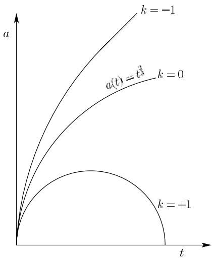
Figure 18.5 Friedmann cosmological models

Observational cosmology is still trying to decide which of these models is the closest representation of our actual universe, but most evidence favours the open model.

Problems

Problem 18.28

Show that for a closed Friedmann model of total mass $M$, the maximum radius is reached at $t=2GM/3c^3$ where its value is $a_{\max }=4GM/3\pi c^2$

Problem 18.29

Show that the radiationfilled universe, $\begin{array}{r}P=\frac{1}{3}\rho \end{array}$ has $\rho \propto a^{-4}$ and the time evolution for $k=0$ is given by $a\propto t^{1/2}$ . Assuming the radiation is black body, $\rho =a_S{T}^4$ , where $a_S=7.55\times 10^{-15}\mathrm{erg}{\mathrm{cm}}^{-3}{\mathrm{K}}^{-4}$ , show that the temperature of the universe evolves with time as

$$T={\left(\frac{3c^2}{32\pi G{a}_S}\right)}^{1/4}{t}^{-1/2}=\frac{1.52}{\sqrt{t}}\mathrm{K}(t\text{ in seconds }).$$

Problem 18.30

Consider two radial light signals (null geodesics) received at the spatial origin of coordinates at times $t_0$ and $t_0+\Delta t_0$ , emitted from $\chi ={\chi }_1(\mathrm{or}r=r_1$ in the case of the flat models) at time $t=t_1<t_0$ . By comparing proper times between reception and emission show that the observer experiences a redshift in the case of an expanding universe ($a$($t$) increasing) given by

$$1+z=\frac{\Delta t_0}{\Delta t_1}=\frac{a(t_0)}{a(t_1)}.$$

Problem 18.31

By considering light signals as in the previous problem, show that an observer at $r=0.$ , in the Einstein–de Sitter universe can at time $t=t_0$ see no events having radial coordinate $r>r_H=3c{t}_0$ . Show that the mass contained within this radius, called the particle horizon, is given by $M_H=6c^3{t}_0/G$