7.2 Parallel transport, connection and covariant derivative

A vector $X$ is a directional derivative acting on $f\in \mathcal{F}(M)$ as $X:f\mapsto X[f]$ . However, there is no directional derivative acting on a tensor field of type $(p,q)$ , which arises naturally from the differentiable structure of $M$ . [Note that the Lie derivative ${\mathcal{L}}_{V}X=[V,X]$ is not a directional derivative since it depends on the derivative of $V$ .] What we need is an extra structure called the connection, which specifies how tensors are transported along a curve.

7.2.1 Heuristic introduction

We first give a heuristic approach to parallel transport and covariant derivatives. As we have noted several times, two vectors defined at different points cannot be compared naively with each other. Let us see how the derivative of a vector field in a Euclidean space ${\mathbb{R}}^m$ is defined. The derivative of a vector field $V=V^{\mu }{e}_{\mu }$ with respect to $x^{\nu }$ has the $\mu$ th component

$$\frac{\partial V^{\mu }}{\partial x^{\nu }}=\underset{\Delta x\to 0}{\lim }\frac{V^{\mu }(\dots ,x^{\nu }+\Delta x^{\nu },\dots )-V^{\mu }(\dots ,x^{\nu },\dots )}{\Delta x^{\nu }}.$$

The first term in the numerator of the LHS is defined at $x+\Delta x=(x^1,\dots ,x^{\nu }+\Delta x^{\nu },\dots ,x^m)$ , while the second term is defined at $x=(x^{\mu })$ . To subtract $V^{\mu }(x)$ from $V^{\mu }(x+\Delta x)$ , we have to transport $V^{\mu }(x)$ to $x+\Delta x$ without change and compute the difference. This transport of a vector is called a parallel transport. We have implicitly assumed that $V{|}_x$ parallel transported to $x+\Delta x$ has the same component $V^{\mu }(x)$ . However, there is no natural way to parallel transport a vector in a manifold and we have to specify how it is parallel transported from one point

to the other. Let $\tilde{V}{|}_{x+\Delta x}$ denote a vector $V{|}_x$ parallel transported to $x+\Delta x$ . We demand that the components satisfy

$${\tilde{V}}^{\mu }(x+\Delta x)-V^{\mu }(x)\propto \Delta x\text{\hspace{1em}(7.8a)}$$

$$\left(\widetilde{V^{\mu }+W^{\mu }}\right)(x+\Delta x)={\tilde{V}}^{\mu }(x+\Delta x)+{\tilde{W}}^{\mu }(x+\Delta x).\text{\hspace{1em}(7.8b)}$$

These conditions are satisfied if we take

$${\tilde{V}}^{\mu }(x+\Delta x)=V^{\mu }(x)-V^{\lambda }(x){\Gamma }_{\nu \lambda }^{\mu }(x)\Delta x^{\nu }.\text{\hspace{1em}(7.9)}$$

The covariant derivative of $V$ with respect to $x^{\nu }$ is defined by

$$\underset{\Delta x^v\to 0}{\lim }\frac{V^{\mu }(x+\Delta x)-{\tilde{V}}^{\mu }(x+\Delta x)}{\Delta x^v}\frac{\partial }{\partial x^{\mu }}=\left(\frac{\partial V^{\mu }}{\partial x^v}+V^{\lambda }{\Gamma }_{v\lambda }^{\mu }\right)\frac{\partial }{\partial x^{\mu }}.\text{\hspace{1em}(7.10)}$$

This quantity is a vector at $x+\Delta x$ since it is a difference of two vectors $V{|}_{x+\Delta x}$ and $\tilde{V}{|}_{x+\Delta x}$ defined at the same point $x+\Delta x$ . There are many distinct rules of parallel transport possible, one for each choice of $\Gamma$ . If the manifold is endowed with a metric, there exists a preferred choice of $\Gamma$ , called the Levi-Civita connection, see example 7.1 and section 7.4.

Example 7.1

Let us work out a simple example: two-dimensional Euclidean space $({\mathbb{R}}^2,\delta )$ . We define parallel transportation according to the usual sense in elementary geometry. In the Cartesian coordinate system $(x,y)$ , all the components of $\Gamma$ vanish since ${\tilde{V}}^{\mu }(x+\Delta x,y+\Delta y)=V^{\mu }(x,y)$ for any $\Delta x$ and $\Delta y$ . Next we take the polar coordinates $(r,\varphi )$ . If $(r,\varphi )\mapsto (r\cos \varphi ,r\sin \varphi )$ is regarded as an embedding, we find the induced metric,

$$g=\mathrm{d}r\otimes \mathrm{d}r+r^2\mathrm{d}\varphi \otimes \mathrm{d}\varphi .\text{\hspace{1em}(7.11)}$$

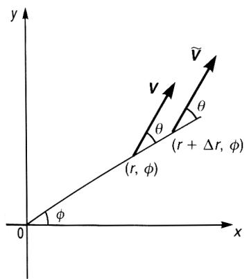
Let $V=V^r\partial /\partial r+V^{\varphi }\partial /\partial \varphi$ be a vector defined at $(r,\varphi )$ . If we parallel transport this vector to $(r+\Delta r,\varphi )$ , we have a new vector $\tilde{V}={\tilde{V}}^r\partial /\partial r{|}_{(r+\Delta r,\varphi )}+{\tilde{V}}^{\varphi }\partial /\partial \varphi {|}_{(r+\Delta r,\varphi )}$ (figure 7.1(a)). Note that $V^r=V\cos \theta$ and $V^{\varphi }=V(\sin \theta /r)$ , where $V=\sqrt{g(\overline{V},\overline{V})}$ and $\theta$ is the angle between $V$ and $\partial /\partial r$ . Then we have ${\tilde{V}}^r=V^r$ and

(a)

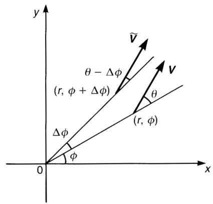
(b)

Figure 7.1. $\tilde{V}$ is a vector $V$ parallel transported to $(a)(r+\Delta r,\varphi )$ and $(b)(r,\varphi +\Delta \varphi )$ .

$${\tilde{V}}^{\varphi }=\frac{r}{r+\Delta r}{V}^{\varphi }\simeq V^{\varphi }-\frac{\Delta r}{r}{V}^{\varphi }.$$

By comparing these components with (7.9), we easily find that

$${\Gamma }_{rr}^r=0{\Gamma }_{r\varphi }^r=0{\Gamma }_{rr}^{\varphi }=0{\Gamma }_{r\varphi }^{\varphi }=\frac{1}{r}.\text{\hspace{1em}(7.12a)}$$

Similarly, if $V$ is parallel transported to $(r,\varphi +\Delta \varphi )$ , it becomes

$$\tilde{V}={\tilde{V}}^r\frac{\partial }{\partial r}{|}_{(r,\varphi +\Delta \varphi )}+{\tilde{V}}^{\varphi }\frac{\partial }{\partial \varphi }{|}_{(r,\varphi +\Delta \varphi )}$$

where

$${\tilde{V}}^r=V\cos (\theta -\Delta \varphi )\simeq V\cos \theta +V\sin \theta \Delta \varphi =V^r+V^{\varphi }r\Delta \varphi$$

and

$${\tilde{V}}^{\varphi }=V\frac{\sin (\theta -\Delta \varphi )}{r}\simeq V\frac{\sin \theta }{r}-V\cos \theta \frac{\Delta \varphi }{r}=V^{\varphi }-V^r\frac{\Delta \varphi }{r}$$

(figure 7.1(b)). Then we find

$${\Gamma }_{\varphi r}^r=0{\Gamma }_{\varphi \varphi }^r=-r{\Gamma }_{\varphi r}^{\varphi }=\frac{1}{r}{\Gamma }_{\varphi \varphi }^{\varphi }=0.\text{\hspace{1em}(7.12b)}$$

Note that the $\Gamma$ satisfy the symmetry ${\Gamma }_{\mu \nu }^{\lambda }={\Gamma }_{\nu \mu }^{\lambda }$ . It is also implicitly assumed that the norm of a vector is invariant under parallel transport. A rule of parallel transport which satisfies these two conditions is called a Levi-Civita connection, see section 7.4. Our intuitive approach leads us to the formal definition of the affine connection.

7.2.2 Affine connections

Definition 7.2

An affine connection $\nabla$ is a map $\nabla :\mathcal{X}(M)\times \mathcal{X}(M)\to \mathcal{X}(M)$ , or $(X,Y)\mapsto {\nabla }_{X}Y$ which satisfies the following conditions:

$${\nabla }_X(Y+Z)={\nabla }_{X}Y+{\nabla }_{X}Z\text{\hspace{1em}(7.13a)}$$

$${\nabla }_{(X+Y)}Z={\nabla }_{X}Z+{\nabla }_{Y}Z\text{\hspace{1em}(7.13b)}$$

$${\nabla }_{(fX)}Y=f{\nabla }_{X}Y\text{\hspace{1em}(7.13c)}$$

$${\nabla }_X(fY)=X[f]Y+f{\nabla }_{X}Y\text{\hspace{1em}(7.13d)}$$

where $f\in \mathcal{F}(M)$ and $X,Y,Z\in \mathcal{X}(M)$

Take a chart $(U,\phi )$ with the coordinate $x=\phi (p)$ on $M$ , and define $m^3$ functions ${\Gamma }_{\nu \mu }^{\lambda }$ called the connection coefficients by

$${\nabla }_v{e}_{\mu }\equiv {\nabla }_{e_v}{e}_{\mu }=e_{\lambda }{\Gamma }_{v\mu }^{\lambda }\text{\hspace{1em}(7.14)}$$

where $\{e_{\mu }\}=\{\partial /\partial x^{\mu }\}$ is the coordinate basis in $T_{p}M$ . The connection coefficients specify how the basis vectors change from point to point. Once the action of $\nabla$ on the basis vectors is defined, we can calculate the action of $\nabla$ on any vectors. Let $V=V^{\mu }{e}_{\mu }$ and $W=W^{\nu }{e}_{\nu }$ be elements of $T_p(M)$ . Then

$$\begin{array}{rl}{\nabla }_{V}W& =V^{\mu }{\nabla }_{e_{\mu }}\left(W^v{e}_v\right)=V^{\mu }\left(e_{\mu }\left[W^{\mu }\right]e_v+W^v{\nabla }_{e_{\mu }}{e}_v\right)\\ & =V^{\mu }\left(\frac{\partial W^{\lambda }}{\partial x^{\mu }}+W^v{\Gamma }_{\mu v}^{\lambda }\right)e_{\lambda }.\end{array}\text{\hspace{1em}(7.15)}$$

Note that this definition of the connection coefficient is in agreement with the previous heuristic result (7.10). By definition, $\nabla$ maps two vectors $V$ and $W$ to a new vector given by the RHS of (7.15), whose $\lambda$ th component is $V^{\mu }{\nabla }_{\mu }{W}^{\lambda }$ where

$${\nabla }_{\mu }{W}^{\lambda }\equiv \frac{\partial W^{\lambda }}{\partial x^{\mu }}+{\Gamma }_{\mu v}^{\lambda }{W}^v.\text{\hspace{1em}(7.16)}$$

Note that ${\nabla }_{\mu }{W}^{\lambda }$ is the $\lambda$ th component of a vector ${\nabla }_{\mu }W={\nabla }_{\mu }{W}^{\lambda }{e}_{\lambda }$ and should not be confused with the covariant derivative of a component $W^{\lambda }$ . ${\nabla }_{V}W$ is independent of the derivative of $V$ , unlike the Lie derivative ${\mathcal{L}}_{V}W=[V,W]$ . In this sense, the covariant derivative is a proper generalization of the directional derivative of functions to tensors.

7.2.3 Parallel transport and geodesics

Given a curve in a manifold $M$ , we may define the parallel transport of a vector along the curve. Let $c:(a,b)\to M$ be a curve in $M$ . For simplicity, we assume the image is covered by a single chart $(U,\phi )$ whose coordinate is $x=\phi (p)$ . Let $X$ be a vector field defined (at least) along $c(t)$ ,

$$X{\mid }_{c(t)}=X^{\mu }(c(t))e_{\mu }{\mid }_{c(t)}\text{\hspace{1em}(7.17)}$$

where $e_{\mu }=\partial /\partial x^{\mu }$ . If $X$ satisfies the condition

$${\nabla }_{V}X=0\text{f o r a n y}t\in (a,b)\text{\hspace{1em}(7.18a)}$$

$X$ is said to be parallel transported along $c(t)$ where $V=\mathrm{d}/\mathrm{dt}=({\mathrm{dx}}^{\mu }(c(t))/\mathrm{dt})e_{\mu }{|}_{c(t)}$ is the tangent vector to $c(t)$ . The condition (7.18a) is written in terms of the components as

$$\frac{\mathrm{d}{X}^{\mu }}{\mathrm{d}t}+{\Gamma }_{\nu \lambda }^{\mu }\frac{\mathrm{d}{x}^{\nu }(c(t))}{\mathrm{d}t}{X}^{\lambda }=0.\text{\hspace{1em}(7.18b)}$$

If the tangent vector $V(t)$ itself is parallel transported along $c(t)$ , namely if

$${\nabla }_{V}V=0\text{\hspace{1em}(7.19a)}$$

the curve $c(t)$ is called a geodesic. Geodesics are, in a sense, the straightest possible curves in a Riemannian manifold. In components, the geodesic equation (7.19a) becomes

$$\frac{{\mathrm{d}}^2{x}^{\mu }}{\mathrm{d}{t}^2}+{\Gamma }_{\nu \lambda }^{\mu }\frac{\mathrm{d}{x}^{\nu }}{\mathrm{d}t}\frac{\mathrm{d}{x}^{\lambda }}{\mathrm{d}t}=0\text{\hspace{1em}(7.19b)}$$

where $\{x^{\mu }\}$ are the coordinates of $c(t)$ . We might say that (7.19a) is too strong to be the condition for the straightest possible curve, and instead require a weaker condition

$${\nabla }_{V}V=fV\text{\hspace{1em}(7.20)}$$

where $f\in \mathcal{F}(M)$ . ‘Change of $V$ is parallel to $V$ ’ is also a feature of a straight line. However, under the reparametrization $t\to t^{\prime }$ , the component of the tangent vector changes as

$$\frac{\mathrm{d}{x}^{\mu }}{\mathrm{d}t}\to \frac{\mathrm{d}t}{\mathrm{d}{t}^{\prime }}\frac{\mathrm{d}{x}^{\mu }}{\mathrm{d}t}$$

and (7.20) reduces to (7.19a) if $t^{\prime }$ satisfies

$$\frac{{\mathrm{d}}^2{t}^{\prime }}{\mathrm{d}{t}^2}=f\frac{\mathrm{d}{t}^{\prime }}{\mathrm{d}t}.$$

Thus, it is always possible to reparametrize the curve so that the geodesic equation takes the form (7.19a).

Exercise 7.3

Show that (7.19b) is left invariant under the affine reparametrization $t\to at+b$ ( $a,b\in \mathbb{R}$ ).

7.2.4 The covariant derivative of tensor fields

Since ${\nabla }_X$ has the meaning of a derivative, it is natural to define the covariant derivative of $f\in \mathcal{F}(M)$ by the ordinary directional derivative:

$${\nabla }_{X}f=X[f].\text{\hspace{1em}(7.21)}$$

Then (7.13d) looks exactly like the Leibnitz rule,

$${\nabla }_X(fY)=({\nabla }_{X}f)Y+f{\nabla }_{X}Y.\text{\hspace{1em}(7.13d’)}$$

We require that this be true for any product of tensors,

$${\nabla }_X\left(T_1\otimes T_2\right)=\left({\nabla }_X{T}_1\right)\otimes T_2+T_1\otimes \left({\nabla }_X{T}_2\right)\text{\hspace{1em}(7.22)}$$

where $T_1$ and $T_2$ are tensor fields of arbitrary types. Equation (7.22) is also true when some of the indices are contracted. With these requirements, we compute the covariant derivative of a one-form $\omega \in {\Omega }^1(M)$ . Since $⟨\omega ,Y⟩\in \mathcal{F}(M)$ for $Y\in \mathcal{X}(M)$ , we should have

$$X[⟨\omega ,Y⟩]={\nabla }_X[⟨\omega ,Y⟩]=⟨{\nabla }_X\omega ,Y⟩+⟨\omega ,{\nabla }_{X}Y⟩.$$

Writing down both sides in terms of the components we find

$$({\nabla }_X\omega {)}_v=X^{\mu }{\partial }_{\mu }{\omega }_v-X^{\mu }{\Gamma }_{\mu v}^{\lambda }{\omega }_{\lambda }.\text{\hspace{1em}(7.23)}$$

In particular, for $X=e_{\mu }$ , we have

$$({\nabla }_{\mu }\omega {)}_v={\partial }_{\mu }{\omega }_v-{\Gamma }_{\mu v}^{\lambda }{\omega }_{\lambda }.\text{\hspace{1em}(7.24)}$$

For $\omega =\mathrm{d}{x}^{\nu }$ , we obtain (cf (7.14))

$${\nabla }_{\mu }\mathrm{d}{x}^{\nu }=-{\Gamma }_{\mu \lambda }^{\nu }\mathrm{d}{x}^{\lambda }.\text{\hspace{1em}(7.25)}$$

It is easy to generalize these results as

$$\begin{array}{rl}& {\nabla }_{\nu }{t}_{{\mu }_1\dots {\mu }_q}^{{\lambda }_1\dots {\lambda }_p}={\partial }_{\nu }{t}_{{\mu }_1\dots {\mu }_q}^{{\lambda }_1\dots {\lambda }_p}+{\Gamma }_{\nu \kappa }^{{\lambda }_1}{t}_{{\mu }_1\dots {\mu }_q}^{\kappa {\lambda }_2\dots {\lambda }_p}+\dots \\ & +{\Gamma }_{\nu \kappa }^{{\lambda }_p}{t}_{{\mu }_1\dots {\mu }_q}^{{\lambda }_1\dots {\lambda }_{p-1}\kappa }-{\Gamma }_{\nu {\mu }_1}^{\kappa }{t}_{\kappa {\mu }_2\dots {\mu }_q}^{{\lambda }_1\dots {\lambda }_p}-\dots \\ & -{\Gamma }_{v{\mu }_q}^{\kappa }{t}_{{\mu }_1\dots {\mu }_{q-1}\kappa }^{{\lambda }_1\dots {\lambda }_p}.\end{array}\text{\hspace{1em}(7.26)}$$

Exercise 7.4

Let $g$ be a metric tensor. Verify that

$$({\nabla }_{v}g{)}_{\lambda \mu }={\partial }_v{g}_{\lambda \mu }-{\Gamma }_{v\lambda }^{\kappa }{g}_{\kappa \mu }-{\Gamma }_{v\mu }^{\kappa }{g}_{\lambda \kappa }.\text{\hspace{1em}(7.27)}$$

7.2.5 The transformation properties of connection coefficients

Introduce another chart $(V,\psi )$ such that $U\cap V\ne \varnothing$ , whose coordinates are $y=\psi (p)$ . Let $\{e_{\mu }\}=\{\partial /\partial x^{\mu }\}$ and $\{f_{\alpha }\}=\{\partial /\partial y^{\alpha }\}$ be bases of the respective coordinates. Denote the connection coefficients with respect to the $y$ -coordinates by ${\tilde{\Gamma }}_{\beta \gamma }^{\alpha }$ . The basis vector $f_{\alpha }$ satisfies

$${\nabla }_{f_{\alpha }}{f}_{\beta }={\tilde{\Gamma }}_{\alpha \beta }^{\gamma }{f}_{\gamma }.\text{\hspace{1em}(7.28)}$$

If we write $f_{\alpha }=(\partial x^{\mu }/\partial y^{\alpha })e_{\mu }$ , the LHS becomes

$$\begin{array}{rl}{\nabla }_{f_{\alpha }}{f}_{\beta }& ={\nabla }_{f_{\alpha }}\left(\frac{\partial x^{\mu }}{\partial y^{\beta }}{e}_{\mu }\right)=\frac{{\partial }^2{x}^{\mu }}{\partial y^{\alpha }\partial y^{\beta }}{e}_{\mu }+\frac{\partial x^{\lambda }}{\partial y^{\alpha }}\frac{\partial x^{\mu }}{\partial y^{\beta }}{\nabla }_{e_{\lambda }}{e}_{\mu }\\ & =\left(\frac{{\partial }^2{x}^{\nu }}{\partial y^{\alpha }\partial y^{\beta }}+\frac{\partial x^{\lambda }}{\partial y^{\alpha }}\frac{\partial x^{\mu }}{\partial y^{\beta }}{\Gamma }_{\lambda \mu }^{\nu }\right)e_{\nu }.\end{array}$$

Since the RHS of (7.28) is equal to ${\tilde{\Gamma }}_{\alpha \beta }^{\gamma }(\partial x^{\nu }/\partial y^{\gamma })e_{\nu }$ , the connection coefficients must transform as

$${\tilde{\Gamma }}_{\alpha \beta }^{\gamma }=\frac{\partial x^{\lambda }}{\partial y^{\alpha }}\frac{\partial x^{\mu }}{\partial y^{\beta }}\frac{\partial y^{\gamma }}{\partial x^{\nu }}{\Gamma }_{\lambda \mu }^{\nu }+\frac{{\partial }^2{x}^{\nu }}{\partial y^{\alpha }\partial y^{\beta }}\frac{\partial y^{\gamma }}{\partial x^{\nu }}.\text{\hspace{1em}(7.29)}$$

The reader should verify that this transformation rule indeed makes ${\nabla }_{X}Y$ a vector, namely

$${\tilde{X}}^{\alpha }\left({\tilde{\partial }}_{\alpha }{\tilde{Y}}^{\gamma }+{\tilde{\Gamma }}_{\alpha \beta }^{\gamma }{\tilde{Y}}^{\beta }\right)f_{\gamma }=X^{\lambda }\left({\partial }_{\lambda }{Y}^{\nu }+{\Gamma }_{\lambda \mu }^{\nu }{Y}^{\nu }\right)e_{\nu }.$$

In the literature, connection coefficients are often defined as objects which transform as (7.29). From our viewpoint, however, they must transform according to (7.29) to make ${\nabla }_{X}Y$ independent of the coordinate chosen.

Exercise 7.5

Let $\Gamma$ be an arbitrary connection coefficient. Show that ${\Gamma }_{\mu \nu }^{\lambda }+t_{\mu \nu }^{\lambda }$ is another connection coefficient provided that $t_{\mu \nu }^{\lambda }$ is a tensor field. Conversely, suppose ${\Gamma }_{\mu \nu }^{\lambda }$ and ${\bar{\Gamma }}_{\mu \nu }^{\lambda }$ are connection coefficients. Show that ${\Gamma }_{\mu \nu }^{\lambda }-{\bar{\Gamma }}_{\mu \nu }^{\lambda }$ is a component of a tensor of type (1, 2).

7.2.6 The metric connection

So far we have left $\Gamma$ arbitrary. Now that our manifold is endowed with a metric, we may put reasonable restrictions on the possible form of connections. We demand that the metric $g_{\mu \nu }$ be covariantly constant, that is, if two vectors $X$ and $Y$ are parallel transported along any curve, then the inner product between them remains constant under parallel transport. [In example 7.1, we have already assumed this reasonable condition.] Let $V$ be a tangent vector to an arbitrary curve along which the vectors are parallel transported. Then we have

$$\begin{array}{rl}0& ={\nabla }_V[g(X,Y)]=V^K[({\nabla }_{\kappa }g)(X,Y)+g({\nabla }_{\kappa }X,Y)+g(X,{\nabla }_{\kappa }Y)]\\ & =V^{\kappa }{X}^{\mu }{Y}^{\nu }({\nabla }_{\kappa }g{)}_{\mu \nu }\end{array}$$

where we have noted that ${\nabla }_{\kappa }X={\nabla }_{\kappa }Y=0$ . Since this is true for any curves and vectors, we must have

$$({\nabla }_{\kappa }g{)}_{\mu \nu }=0\text{\hspace{1em}(7.30a)}$$

or, from exercise 7.4,

$${\partial }_{\lambda }{g}_{\mu \nu }-{\Gamma }_{\lambda \mu }^{\kappa }{g}_{\kappa \nu }-{\Gamma }_{\lambda \nu }^{\kappa }{g}_{\kappa \mu }=0.\text{\hspace{1em}(7.30b)}$$

If (7.30a) is satisfied, the affine connection $\nabla$ is said to be metric compatible or simply a metric connection. We will deal with metric connections only. Cyclic permutations of $(\lambda ,\mu ,\nu )$ yield

$$\begin{array}{rl}& {\partial }_{\mu }{g}_{v\lambda }-{\Gamma }_{\mu v}^{\kappa }{g}_{\kappa \lambda }-{\Gamma }_{\mu \lambda }^{\kappa }{g}_{\kappa v}=0(7.30c)\\ & {\partial }_{\nu }{g}_{\lambda \mu }-{\Gamma }_{v\lambda }^{\kappa }{g}_{\kappa \mu }-{\Gamma }_{v\mu }^{\kappa }{g}_{\kappa \lambda }=0.(7.30d)\end{array}$$

The combination $-(7.30\mathrm{b})+(7.30\mathrm{c})+(7.30\mathrm{d})$ yields

$$-{\partial }_{\lambda }{g}_{\mu v}+{\partial }_{\mu }{g}_{\nu \lambda }+{\partial }_v{g}_{\lambda \mu }+T_{\lambda \mu }^{\kappa }{g}_{\kappa v}+T_{\lambda v}^{\kappa }{g}_{\kappa \mu }-2{\Gamma }_{(\mu v)g_{\kappa \lambda }}^{\kappa }=0\text{\hspace{1em}(7.31)}$$

where $T_{\lambda \mu }^{\kappa }\equiv 2{\Gamma }_{[\lambda \mu ]}^{\kappa }\equiv {\Gamma }_{\lambda \mu }^{\kappa }-{\Gamma }_{\mu \lambda }^{\kappa }$ and ${\Gamma }_{(\mu \nu )}^{\kappa }\equiv \frac{1}{2}({\Gamma }_{\nu \mu }^{\kappa }+{\Gamma }_{\mu \nu }^{\kappa })$ . The tensor $T_{\lambda \mu }^{\kappa }$ is anti-symmetric with respect to the lower indices $T_{\lambda \mu }^{\kappa }=-T_{\mu \lambda }^{\kappa }$ and called the torsion tensor, see exercise 7.6. The torsion tensor will be studied in detail in the next section. Equation (7.31) is solved for ${\Gamma }_{(\mu \nu )}^{\kappa }$ to yield

$${\Gamma }_{(\mu \nu )}^{\kappa }=\left\{\begin{array}{l}\kappa \\ \mu \nu \end{array}\right\}+\frac{1}{2}\left(T_{\nu }{}^{\kappa }{}_{\mu }+T_{\mu }{}^{\kappa }{}_{\nu }\right)\text{\hspace{1em}(7.32)}$$

where $\{{\kappa }_{\mu \nu }\}$ are the Christoffel symbols defined by

$$\left\{\begin{array}{c}\kappa \\ \mu v\end{array}\right\}=\frac{1}{2}{g}^{\kappa \lambda }\left({\partial }_{\mu }{g}_{v\lambda }+{\partial }_v{g}_{\mu \lambda }-{\partial }_{\lambda }{g}_{\mu v}\right).\text{\hspace{1em}(7.33)}$$

Finally, the connection coefficient $\Gamma$ is given by

$$\begin{array}{rl}{\Gamma }_{\mu \nu }^{\kappa }& ={\Gamma }_{(\mu \nu )}^{\kappa }+{\Gamma }_{[\mu \nu ]}^{\kappa }\\ & =\left\{\begin{array}{l}\kappa \\ \mu v\end{array}\right\}+\frac{1}{2}\left(T_v{}^{\kappa }{}_{\mu }+T_{\mu }{}^{\kappa }{}_v+T_{\mu v}^{\kappa }\right).\end{array}\text{\hspace{1em}(7.34)}$$

The second term of the last expression of (7.34) is called the contour, denoted by $K_{\mu \nu }^{\kappa }$ :

$$K_{\mu \nu }^{\kappa }\equiv \frac{1}{2}\left(T_{\mu \nu }^{\kappa }+T_{\mu \nu }^{\kappa }+T_{\nu \mu }^{\kappa }\right).\text{\hspace{1em}(7.35)}$$

If the torsion tensor vanishes on a manifold $M$ , the metric connection $\nabla$ is called the Levi-Civita connection. Levi-Civita connections are natural generalizations of the connection defined in the classical geometry of surfaces, see section 7.4.

Exercise 7.6

Show that $T_{\mu \nu }^{\kappa }$ obeys the tensor transformation rule. [Hint: Use (7.29).] Show also that $K_{[\mu \nu ]}^{\kappa }=\frac{1}{2}{T}_{\mu \nu }^{\kappa }$ and $K_{\kappa \mu \nu }=-K_{\nu \mu \kappa }$ where $K_{\kappa \mu \nu }=g_{\kappa \lambda }{K}_{\mu \nu }^{\lambda }$ .

来源与版本

正文：英文 · OCR 机器稿 · 待校对

核对状态：OCR 机器稿 · 待校对

原书 PDF

来源版本：second-edition-local

来源 PDF SHA-256：fcd24c3371d092a8c699ccf5cf0765462924b6c48412804231076e8084b1940d

OCR 来源 SHA-256：0b6324f01172a3548cd34382e82fd8bfae574602b6b2cfaa357ba96bc2c35478

OCR 产物 SHA-256：3473117c1029d729c2cfaa7a8e2ce4d02f339a16e888f9a2716b2defdeff01a7