7.4 Levi-Civita connections

7.4.1 The fundamental theorem

Among affine connections, there is a special connection called the Levi-Civita connection, which is a natural generalization of the connection in the classical differential geometry of surfaces. A connection $\nabla$ is called a symmetric connection if the torsion tensor vanishes. In the coordinate basis, connection coefficients of a symmetric connection satisfy

$${\Gamma }_{\mu \nu }^{\lambda }={\Gamma }_{\nu \mu }^{\lambda }.\text{\hspace{1em}(7.52)}$$

Theorem 7.1 · The fundamental theorem of (pseudo-)Riemannian geometry

On a (pseudo-)Riemannian manifold $(M,g)$ , there exists a unique symmetric connection which is compatible with the metric $g$ . This connection is called the Levi-Civita connection.

Proof

This follows directly from (7.34). Let $\nabla$ be an arbitrary connection such that

$${\tilde{\Gamma }}_{\mu v}^{\kappa }=\left\{\begin{array}{c}\kappa \\ \mu v\end{array}\right\}+K_{\mu v}^{\kappa }$$

where $\left\{\begin{array}{c}\kappa \\ \mu \nu \end{array}\right\}$ is the Christoffel symbol and $K$ the contorsion tensor. It was shown in exercise 7.5 that ${\Gamma }_{\mu \nu }^{\kappa }\equiv {\tilde{\Gamma }}_{\mu \nu }^{\kappa }+t_{\mu \nu }^{\kappa }$ is another connection coefficient if $t$ is a tensor field of type (1, 2). Now we choose $t_{\mu \nu }^{\kappa }=-K_{\mu \nu }^{\kappa }$ so that

$${\Gamma }_{\mu \nu }^{\kappa }=\left\{\begin{array}{l}\kappa \\ \mu \nu \end{array}\right\}=\frac{1}{2}{g}^{\kappa \lambda }\left({\partial }_{\mu }{g}_{\lambda \nu }+{\partial }_{\nu }{g}_{\lambda \mu }-{\partial }_{\lambda }{g}_{\mu \nu }\right).\text{\hspace{1em}(7.53)}$$

By construction, this is symmetric and certainly unique given a metric.

Exercise 7.8

Let $V$ be a Levi-Civita connection.

(a) Let $f\in \mathcal{F}(M)$ . Show that

$${\nabla }_{\mu }{\nabla }_{\nu }f={\nabla }_{\nu }{\nabla }_{\mu }f.\text{\hspace{1em}(7.54)}$$

(b) Let $\omega \in {\Omega }^1(M)$ . Show that

$$\mathrm{d}\omega =({\nabla }_{\mu }\omega {)}_{\nu }\mathrm{d}{x}^{\mu }\wedge \mathrm{d}{x}^{\nu }.\text{\hspace{1em}(7.55)}$$

(c) Let $\omega \in {\Omega }^1(M)$ and let $U\in \mathcal{X}(M)$ be the corresponding vector field: $U^{\mu }=g^{\mu \nu }{\omega }_{\nu }$ . Show that, for any $V\in \mathcal{X}(M)$ ,

$$g\left({\nabla }_{X}U,V\right)=⟨{\nabla }_X\omega ,V⟩.\text{\hspace{1em}(7.56)}$$

(a) The metric on ${\mathbb{R}}^2$ in polar coordinates is $g=\mathrm{d}r\otimes \mathrm{d}r+r^2\mathrm{d}\varphi \otimes \mathrm{d}\varphi$ . The non-vanishing components of the Levi-Civita connection coefficients are ${\Gamma }_{r\varphi }^{\varphi }={\Gamma }_{\varphi r}^{\varphi }=r^{-1}$ and ${\Gamma }_r{}^{\varphi }{}_{\varphi }=-r$ . This is in agreement with the result obtained in example 7.1.
(b) The induced metric on $S^2$ is $g=\mathrm{d}\theta \otimes \mathrm{d}\theta +{\sin }^2\theta \mathrm{d}\varphi \otimes \mathrm{d}\varphi$ . The nonvanishing components of the Levi-Civita connection are

$${\Gamma }_{\varphi \varphi }^{\theta }=-\cos \theta \sin \theta {\Gamma }_{\theta \varphi }^{\varphi }={\Gamma }_{\varphi \theta }^{\varphi }=\cot \theta .\text{\hspace{1em}(7.57)}$$

7.4.2 The Levi-Civita connection in the classical geometry of surfaces

In the classical differential geometry of surfaces embedded in ${\mathbb{R}}^3$ , Levi-Civita defined the parallelism of vectors at the nearby points $p$ and $q$ in the following sense (figure 7.6). First, take the tangent plane at $p$ and a vector $V_p$ at $p$ , which lies in the tangent plane. A vector $V_q$ at $q$ is defined to be parallel to $V_p$ if the projection of $V_q$ to the tangent plane at $p$ is parallel to $V_p$ in our usual sense. Now take two points $q$ and $s$ near $p$ as in figure 7.7 and parallel transport the displacement vectors $pq$ along $ps$ and $ps$ along $pq$ . If the parallelism is defined in the sense of Levi-Civita, the displacement vectors projected to the tangent plane at $p$ form a closed parallelogram, hence this parallelism has vanishing torsion. As has been proved in theorem 7.1, there exists a unique connection which has vanishing torsion, which generalizes the parallelism defined here to arbitrary manifolds.

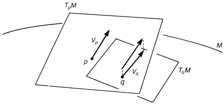
Figure 7.6. On a surface $M$ , a vector $V_p\in T_{p}M$ is defined to be parallel to $V_q\in T_{q}M$ if the projection of $V_q$ onto $T_{p}M$ is parallel to $V_p$ in our ordinary sense of parallelism in ${\mathbb{R}}^2$ .

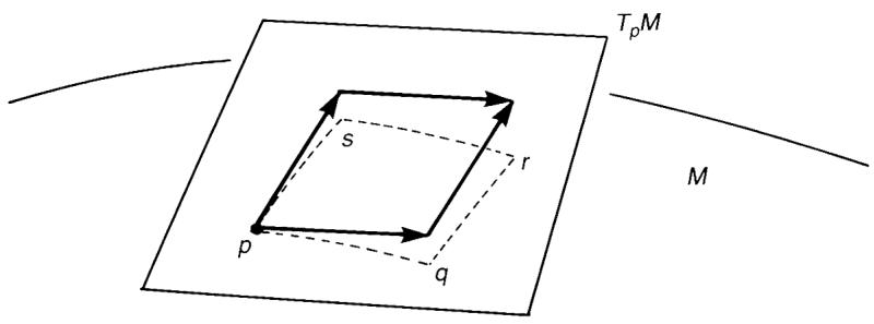
Figure 7.7. If the parallelism is defined in the sense of Levi-Civita, the torsion vanishes identically.

7.4.3 Geodesics

When the Levi-Civita connection is employed, we can compute the connection coefficients, Riemann tensors and many relations involving these by simple routines. Besides this simplicity, the Levi-Civita connection provides a geodesic (defined as the straightest possible curve) with another picture, namely the shortest possible curve connecting two given points. In Newtonian mechanics, the trajectory of a free particle is the straightest possible as well as the shortest possible curve, that is, a straight line. Einstein proposed that this property should be satisfied in general relativity as well; if gravity is understood as a part of the geometry of spacetime, a freely falling particle should follow the straightest as well as the shortest possible curve. [Remark: To be precise, the shortest possible curve is too strong a condition. As we see later, a geodesic defined with respect to the Levi-Civita connection gives the local extremum of the length of a curve connecting two points.]

Example 7.4

In a flat manifold $({\mathbb{R}}^m,\delta )$ or $({\mathbb{R}}^m,\eta )$ , the Levi-Civita connection coefficients $\Gamma$ vanish identically. Hence, the geodesic equation (7.19b) is easily solved to yield $x^{\mu }=A^{\mu }t+B^{\mu }$ , where $A^{\mu }$ and $B^{\mu }$ are constants.

Exercise 7.9

A metric on a cylinder $S^1\times \mathbb{R}$ is given by $g=\mathrm{d}\varphi \otimes \mathrm{d}\varphi +\mathrm{d}z\otimes \mathrm{d}z$ , where $\varphi$ is the polar angle of $S^1$ and $z$ the coordinate of $\mathbb{R}$ . Show that the geodesics given by the Levi-Civita connection are helices.

The equivalence of the straightest possible curve and the local extremum of the distance is proved as follows. First we parametrize the curve by the distance $s$ along the curve, $x^{\mu }=x^{\mu }(s)$ . The length of a path $c$ connecting two points $p$ and $q$ is

$$I(c)={\int }_c\mathrm{d}s={\int }_c\sqrt{g_{\mu v}{x}^{\prime \mu }{x}^{\prime v}}\mathrm{d}s\text{\hspace{1em}(7.58)}$$

where $x^{\prime \mu }=\mathrm{d}{x}^{\mu }/\mathrm{d}s$ . Instead of deriving the Euler-Lagrange equation from (7.58), we will solve a slightly easier problem. Let $F\equiv \frac{1}{2}{g}_{\mu \nu }{x}^{\prime \mu }{x}^{\prime \nu }$ and write

(7.58) as $I(c)={\int }_{c}L(F)\mathrm{d}s$ . The Euler-Lagrange equation for the original problem takes the form

$$\frac{\mathrm{d}}{\mathrm{d}s}\left(\frac{\partial L}{\partial x^{\prime \lambda }}\right)-\frac{\partial L}{\partial x^{\lambda }}=0.\text{\hspace{1em}(7.59)}$$

Then $F=L^2/2$ satisfies

$$\frac{\mathrm{d}}{\mathrm{d}s}\left(\frac{\partial F}{\partial x^{\prime \lambda }}\right)-\frac{\partial F}{\partial x^{\lambda }}=L\left[\frac{\mathrm{d}}{\mathrm{d}s}\left(\frac{\partial L}{\partial x^{\prime \lambda }}\right)-\frac{\partial L}{\partial x^{\lambda }}\right]+\frac{\partial L}{\partial x^{\prime \lambda }}\frac{\mathrm{d}L}{\mathrm{d}s}=\frac{\partial L}{\partial x^{\prime \lambda }}\frac{\mathrm{d}L}{\mathrm{d}s}.\text{\hspace{1em}(7.60)}$$

The last expression vanishes since $L\equiv 1$ along the curve; $\mathrm{d}L/\mathrm{d}s=0$ . Now we have proved that $F$ also satisfies the Euler-Lagrange equation provided that $L$ does so. We then have

$$\begin{array}{rl}& \frac{\mathrm{d}}{\mathrm{d}s}\left(g_{\lambda \mu }{x}^{\prime \mu }\right)-\frac{1}{2}\frac{\partial g_{\mu v}}{\partial x^{\lambda }}{x}^{\prime \mu }{x}^{\prime v}\\ & =\frac{\partial g_{\lambda \mu }}{\partial x^{\nu }}{x}^{\prime \mu }{x}^{\prime \nu }+g_{\lambda \mu }\frac{{\mathrm{d}}^2{x}^{\mu }}{\mathrm{d}{s}^2}-\frac{1}{2}\frac{\partial g_{\mu \nu }}{\partial x^{\lambda }}{x}^{\prime \mu }{x}^{\prime \nu }\\ & =g_{\lambda \mu }\frac{d^2{x}^{\mu }}{\mathrm{d}{s}^2}+\frac{1}{2}\left(\frac{\partial g_{\lambda \mu }}{\partial x^{\nu }}+\frac{\partial g_{\lambda \nu }}{\partial x^{\mu }}-\frac{\partial g_{\mu \nu }}{\partial x^{\lambda }}\right)\frac{\mathrm{d}{x}^{\mu }}{\mathrm{d}s}\frac{\mathrm{d}{x}^{\nu }}{\mathrm{d}s}=0.\end{array}\text{\hspace{1em}(7.61)}$$

If (7.61) is multiplied by $g^{\kappa \lambda }$ , we reproduce the geodesic equation (7.19b).

Having proved that $L$ and $F$ satisfy the same variational problem, we take advantage of this to compute the Christoffel symbols. Take $S^2$ , for example. $F$ is given by $\frac{1}{2}({\theta }^{\prime 2}+{\sin }^2\theta {\varphi }^{\prime 2})$ and the Euler-Lagrange equations are

$$\frac{{\mathrm{d}}^2\theta }{\mathrm{d}{s}^2}-\sin \theta \cos \theta {\left(\frac{\mathrm{d}\varphi }{\mathrm{d}s}\right)}^2=0\text{\hspace{1em}(7.62a)}$$

$$\frac{{\mathrm{d}}^2\varphi }{\mathrm{d}{s}^2}+2\cot \theta \frac{\mathrm{d}\varphi }{\mathrm{d}s}\frac{\mathrm{d}\theta }{\mathrm{d}s}=0.\text{\hspace{1em}(7.62b)}$$

It is easy to read off the connection coefficients ${\Gamma }_{\varphi \varphi }^{\theta }=-\sin \theta \cos \theta$ and ${\Gamma }_{\varphi \theta }^{\varphi }={\Gamma }_{\theta \varphi }^{\varphi }=\cot \theta$ , see (7.57).

Example 7.5

Let us compute the geodesics of $S^2$ . Rather than solving the geodesic equations (7.62) we find the geodesic by minimizing the length of a curve connecting two points on $S^2$ . Without loss of generality, we may assign coordinates $({\theta }_1,{\varphi }_0)$ and $({\theta }_2,{\varphi }_0)$ to these points. Let $\varphi =\varphi (\theta )$ be a curve connecting these points. Then the length of the curve is

$$I(c)={\int }_{{\theta }_1}^{{\theta }_2}\sqrt{1+{\sin }^2{\left(\frac{\mathrm{d}\varphi }{\mathrm{d}\theta }\right)}^2}\mathrm{d}\theta \text{\hspace{1em}(7.63)}$$

which is minimized when $\mathrm{d}\varphi /\mathrm{d}\theta \equiv 0$ , that is $\varphi \equiv {\varphi }_0$ . Thus, the geodesic is a great circle $(\theta ,{\varphi }_0)$ , ${\theta }_1\le \theta \le {\theta }_2$ . [Remark: Solving (7.62) is not very difficult. Let $\theta =\theta (\varphi )$ be the equation of the geodesic. Then

$$\frac{\mathrm{d}\theta }{\mathrm{d}s}=\frac{\mathrm{d}\theta }{\mathrm{d}\varphi }\frac{\mathrm{d}\varphi }{\mathrm{d}s}\frac{{\mathrm{d}}^2\theta }{\mathrm{d}{s}^2}=\frac{{\mathrm{d}}^2\theta }{\mathrm{d}{\varphi }^2}{\left(\frac{\mathrm{d}\varphi }{\mathrm{d}s}\right)}^2+\frac{\mathrm{d}\theta }{\mathrm{d}\varphi }\frac{{\mathrm{d}}^2\varphi }{\mathrm{d}{s}^2}.$$

Substituting these into the first equation of (7.62), we obtain

$$\frac{{\mathrm{d}}^2\theta }{\mathrm{d}{\varphi }^2}{\left(\frac{\mathrm{d}\varphi }{\mathrm{d}s}\right)}^2+\frac{\mathrm{d}\theta }{\mathrm{d}\varphi }\frac{{\mathrm{d}}^2\varphi }{\mathrm{d}{s}^2}-\sin \theta \cos \theta {\left(\frac{\mathrm{d}\varphi }{\mathrm{d}s}\right)}^2=0.\text{\hspace{1em}(7.64)}$$

The second equation of (7.62) and (7.64) yields

$$\frac{{\mathrm{d}}^2\theta }{\mathrm{d}{\varphi }^2}-2\cot \theta {\left(\frac{\mathrm{d}\theta }{\mathrm{d}\varphi }\right)}^2-\sin \theta \cos \theta =0.\text{\hspace{1em}(7.65)}$$

If we define $f(\theta )\equiv \cot \theta$ (7.65) becomes

$$\frac{{\mathrm{d}}^{2}f}{\mathrm{d}{\varphi }^2}+f=0$$

whose general solution is $f(\theta )=\cot \theta =A\cos \varphi +B\sin \varphi$ or

$$A\sin \theta \cos \varphi +B\sin \theta \sin \varphi -\cos \theta =0.\text{\hspace{1em}(7.66)}$$

Equation (7.66) is the equation of a great circle which lies in a plane whose normal vector is $(A,B,-1)$ .]

Example 7.6

Let $U$ be the upper half-plane $U\equiv \{(x,y)|y>0\}$ and introduce the Poincaré metric

$$g=\frac{\mathrm{d}x\otimes \mathrm{d}x+\mathrm{d}y\otimes \mathrm{d}y}{y^2}.\text{\hspace{1em}(7.67)}$$

The geodesic equations are

$$x^{\prime \prime }-\frac{2}{y}{x}^{\prime }{y}^{\prime }=0\text{\hspace{1em}(7.68a)}$$

$$y^{\prime \prime }-\frac{1}{y}\left[x^{\prime 2}+3y^{\prime 2}\right]=0\text{\hspace{1em}(7.68b)}$$

where $x^{\prime }\equiv \frac{\mathrm{d}x}{\mathrm{d}s}$ etc. The first equation of (7.68) is easily integrated, if divided by $x^{\prime }$ , to yield

$$\frac{x^{\prime }}{y^2}=\frac{1}{R}\text{\hspace{1em}(7.69)}$$

where $R$ is a constant. Since the parameter $s$ is taken so that the vector $(x^{\prime },y^{\prime })$ has unit length, it satisfies $(x^{\prime 2}+y^{\prime 2})/y^2=1$ . From (7.69), this becomes $y^2/R^2+(y^{\prime }/y{)}^2=1$ or

$$\mathrm{d}s=\frac{\mathrm{d}y}{y\sqrt{1-y^2/R^2}}=\frac{\mathrm{d}t}{\sin t}$$

where we put $y=R\sin t$ . Equation (7.69) then becomes

$$x^{\prime }=\frac{y^2}{R}=R{\sin }^{2}t.$$

Now $x$ is solved for $t$ to yield

$$\begin{array}{rl}x& =\int x^{\prime }ds=\int \frac{dx}{ds}\frac{ds}{dt}dt\\ & =\int R\sin tdt=-R\cos t+x_0.\end{array}$$

Finally, we obtain the solution

$$x=-R\cos t+x_{0}y=R\sin t(y>0)\text{\hspace{1em}(7.70)}$$

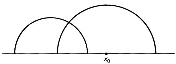
which is a circle with radius $R$ centred at $(x_0,0)$ . Maximally extended geodesics are given by $0<t<\pi$ (figure 7.8) whose length is infinite,

Figure 7.8. Geodesics defined by the Poincaré metric in the upper half-plane. The geodesic has an infinite length.

$$\begin{array}{rl}I& =\int \mathrm{d}s={\int }_{0+\epsilon }^{\pi -\epsilon }\frac{\mathrm{d}s}{\mathrm{d}t}\mathrm{d}t={\int }_{0+\epsilon }^{\pi -\epsilon }\frac{1}{\sin t}\mathrm{d}t\\ & =-\frac{1}{2}\log \frac{1+\cos t}{1-\cos t}{|}_{0+\epsilon }^{\pi -\epsilon }\stackrel{\epsilon \to 0}{\to }\infty .\end{array}$$

7.4.4 The normal coordinate system

The subject here is not restricted to Levi-Civita connections but it does take an especially simple form when the Levi-Civita connection is employed. Let $c(t)$ be

a geodesic in $(M,g)$ defined with respect to a connection $\nabla$ , which satisfies

$$c(0)=p,{\frac{\mathrm{d}}{\mathrm{d}t}|}_p=X=X^{\mu }{e}_{\mu }\in T_{p}M\text{\hspace{1em}(7.71)}$$

where $\{e_{\mu }\}$ is the coordinate basis at $p$ . Any geodesic emanating from $p$ is specified by giving $X\in T_{p}M$ . Take a point $q$ near $p$ . There are many geodesics which connect $p$ and $q$ . However, there exists a unique geodesic $c_q$ such that $c_q(1)=q$ . Let $X_q\in T_{p}M$ be the tangent vector of this geodesic at $p$ . As long as $q$ is not far from $p$ , $q$ uniquely specifies $X_q=X_q^{\mu }{e}_{\mu }\in T_{p}M$ and $\phi :q\to X_q^{\mu }$ serves as a good coordinate system in the neighbourhood of $p$ . This coordinate system is called the normal coordinate system based on $p$ with basis $\{e_{\mu }\}$ . Obviously $\phi (p)=0$ . We define a map $\mathrm{EXP}:T_{p}M\to M$ by $\mathrm{EXP}:X_q\mapsto q$ . By definition, we have

$$\phi \left(\mathrm{EXP}{X}_q^{\mu }{e}_{\mu }\right)=X_q^{\mu }.\text{\hspace{1em}(7.72)}$$

With respect to this coordinate system, a geodesic $c(t)$ with $c(0)=p$ and $c(1)=q$ has the coordinate presentation

$$\phi (c(t))=X^{\mu }=X_q^{\mu }t\text{\hspace{1em}(7.73)}$$

where $X_q^{\mu }$ are the normal coordinates of $q$ .

We now show that Levi-Civita connection coefficients vanish in the normal coordinate system. We write down the geodesic equation in the normal coordinate system,

$$0=\frac{{\mathrm{d}}^2{X}^{\mu }}{\mathrm{d}{t}^2}+{\Gamma }_{v\lambda }^{\mu }\left(X_q^{\kappa }t\right)\frac{\mathrm{d}{X}^v}{\mathrm{d}t}\frac{\mathrm{d}{X}^{\lambda }}{\mathrm{d}t}={\Gamma }_{v\lambda }^{\mu }\left(X_q^{\kappa }t\right)X_q^v{X}_q^{\lambda }.\text{\hspace{1em}(7.74)}$$

Since ${\Gamma }_{\nu \lambda }^{\mu }(p)X_q^{\nu }{X}_q^{\lambda }=0$ for any $X_q^{\nu }$ at $p$ for which $t=0$ , we find ${\Gamma }_{\nu \lambda }^{\mu }(p)+{\Gamma }_{\lambda \nu }^{\mu }(p)=0$ . Since our connection is symmetric we must have

$${\Gamma }_{v\lambda }^{\mu }(p)=0.\text{\hspace{1em}(7.75)}$$

As a consequence, the covariant derivative of any tensor $t$ in this coordinate system takes the extremely simple form at $p$ ,

$${\nabla }_X{t}_{\dots }^{\dots }=X[t_{\dots }^{\dots }].\text{\hspace{1em}(7.76)}$$

Equation (7.75) does not imply that ${\Gamma }_{\nu \lambda }^{\mu }$ vanishes at $q(\ne p)$ . In fact, we find from (7.42) that

$$R_{\lambda \mu \nu }^{\kappa }(p)={\partial }_{\mu }{\Gamma }_{\nu \lambda }^{\kappa }(p)-{\partial }_{\nu }{\Gamma }_{\mu \lambda }^{\kappa }(p)\text{\hspace{1em}(7.77)}$$

hence ${\partial }_{\mu }{\Gamma }_{\nu \lambda }^{\kappa }(p)\ne 0$ if $R_{\lambda \mu \nu }^{\kappa }(p)\ne 0$

7.4.5 Riemann curvature tensor with Levi-Civita connection

Let $\nabla$ be the Levi-Civita connection. The components of the Riemann curvature tensor are given by (7.42) with

$${\Gamma }_{\mu \nu }^{\lambda }=\left\{\begin{array}{c}\kappa \\ \mu \nu \end{array}\right\}$$

while the torsion tensor vanishes by definition. Many formulae are simplified if the Levi-Civita connections are employed.

(a) Let $g=\mathrm{d}r\otimes \mathrm{d}r+r^2(\mathrm{d}\theta \otimes \mathrm{d}\theta +{\sin }^2\theta \mathrm{d}\varphi \otimes \mathrm{d}\varphi )$ be the metric of $({\mathbb{R}}^3,\delta )$ , where $0\le \theta \le \pi$ , $0\le \varphi <2\pi$ . Show, by direct calculation, that all the components of the Riemann curvature tensor with respect to the Levi-Civita connection vanish.

(b) The spatially homogeneous and isotropic universe is described by the Robertson-Walker metric,

$$g=-\mathrm{d}t\otimes \mathrm{d}t+a^2(t)\left(\frac{\mathrm{d}r\otimes \mathrm{d}r}{1-k{r}^2}+r^2(\mathrm{d}\theta \otimes \mathrm{d}\theta +{\sin }^2\theta \mathrm{d}\varphi \otimes \mathrm{d}\varphi )\right)\text{\hspace{1em}(7.78)}$$

where $k$ is a constant, which may be chosen to be $-1$ , 0 or $+1$ by a suitable rescaling of $r$ and $0\le \theta \le \pi$ , $0\le \varphi <2\pi$ . If $k=+1$ , $r$ is restricted to $0\le r<1$ . Compute the Riemann tensor, the Ricci tensor and the scalar curvature.

(c) The Schwarzschild metric takes the form

$$\begin{array}{rl}& g=-\left(1-\frac{2M}{r}\right)dt\otimes dt\\ & +\frac{1}{1-\frac{2M}{r}}dr\otimes dr+r^2(d\theta \otimes d\theta +{\sin }^2\theta d\varphi \otimes d\varphi )\end{array}\text{\hspace{1em}(7.79)}$$

where $0<2M<r$ , $0\le \theta \le \pi$ , $0\le \varphi <2\pi$ . Compute the Riemann tensor, the Ricci tensor and the scalar curvature. [Remark: The metric (7.79) describes a spacetime of a spherically symmetric object with mass $M$ .]

Exercise 7.11

Let $R$ be the Riemann tensor defined with respect to the Levi-Civita connection. Show that

$$\begin{array}{rl}& R_{\kappa \lambda \mu \nu }=\frac{1}{2}\left(\frac{{\partial }^2{g}_{\kappa \mu }}{\partial x^{\lambda }\partial x^{\nu }}-\frac{{\partial }^2{g}_{\lambda \mu }}{\partial x^{\kappa }\partial x^{\nu }}-\frac{{\partial }^2{g}_{\kappa \nu }}{\partial x^{\lambda }\partial x^{\mu }}+\frac{{\partial }^2{g}_{\mu \nu }}{\partial x^{\kappa }\partial x^{\mu }}\right)\\ & +g_{\zeta \eta }\left({\Gamma }_{\kappa \mu }^{\zeta }{\Gamma }_{\lambda \nu }^{\eta }-{\Gamma }_{\kappa \nu }^{\zeta }{\Gamma }_{\lambda \mu }^{\eta }\right)\end{array}$$

where $R_{\kappa \lambda \mu \nu }\equiv g_{\kappa \zeta }{R}_{\lambda \mu \nu }^{\zeta }$ . Verify the following symmetries,

$$R_{\kappa \lambda \mu \nu }=-R_{\kappa \lambda \nu \mu }(\text{c f (7 . 4 3)})\text{\hspace{1em}(7.80a)}$$

$$R_{\kappa \lambda \mu \nu }=-R_{\lambda \kappa \mu \nu }\text{\hspace{1em}(7.80b)}$$

$$R_{\kappa \lambda \mu \nu }=R_{\mu \nu \kappa \lambda }\text{\hspace{1em}(7.80c)}$$

$$Ri{c}_{\mu \nu }=Ri{c}_{v\mu }.\text{\hspace{1em}(7.80d)}$$

Theorem 7.2 · Bianchi identities

Let $R$ be the Riemann tensor defined with respect to the Levi-Civita connection. Then $R$ satisfies the following identities:

$$R(X,Y)Z+R(Z,X)Y+R(Y,Z)X=0$$

(the first Bianchi identity) (7.81a)

$$({\nabla }_{X}R)(Y,Z)V+({\nabla }_{Z}R)(X,Y)V+({\nabla }_{Y}R)(Z,X)V=0$$

(the second Bianchi identity). (7.81b)

Proof

Our proof follows Nomizu (1981). Define the symmetrizer $\mathfrak{S}$ by $\mathfrak{S}\{f(X,Y,Z)\}=f(X,Y,Z)+f(Z,X,Y)+f(Y,Z,X)$ . Let us prove the first Bianchi identity $\mathfrak{S}\{R(X,Y)Z\}=0$ . Covariant differentiation of the identity $T(X,Y)={\nabla }_{X}Y-{\nabla }_{Y}X-[X,Y]=0$ with respect to $Z$ yields

$$\begin{array}{rl}0& ={\nabla }_Z\{{\nabla }_{X}Y-{\nabla }_{Y}X-[X,Y]\}\\ & ={\nabla }_Z{\nabla }_{X}Y-{\nabla }_Z{\nabla }_{Y}X-\left\{{\nabla }_{[X,Y]}Z+[Z,[X,Y]]\right\}\end{array}$$

where the torsion-free condition has been used again to derive the second equality. Symmetrizing this, we have

$$\begin{array}{rl}0& =\mathfrak{S}\left\{{\nabla }_Z{\nabla }_{X}Y-{\nabla }_Z{\nabla }_{Y}X-{\nabla }_{[X,Y]}Z-[Z,[X,Y]]\right\}\\ & =\mathfrak{S}\left\{{\nabla }_Z{\nabla }_{X}Y-{\nabla }_Z{\nabla }_{Y}X-{\nabla }_{[X,Y]}Z\right\}=\mathfrak{S}\left\{R(X,Y)Z\right\}\end{array}$$

where the Jacobi identity $\mathfrak{S}\{[X,[Y,Z]]\}=0$ has been used.

The second Bianchi identity becomes $\mathfrak{S}\{({\nabla }_{X}R)(Y,Z)\}V=0$ where $\mathfrak{S}$ symmetrizes $(X,Y,Z)$ only. If the identity $R(T(X,Y),Z)V=R({\nabla }_{X}Y-{\nabla }_{Y}X-[X,Y],Z)V=0$ is symmetrized, we have

$$\begin{array}{rl}0& =\mathfrak{S}\left\{R\left({\nabla }_{X}Y,Z\right)-R\left({\nabla }_{Y}X,Z\right)-R([X,Y],Z)\right\}V\\ & =\mathfrak{S}\left\{R\left({\nabla }_{Z}X,Y\right)-R(X,{\nabla }_{Z}Y)-R([X,Y],Z)\right\}V.\end{array}\text{\hspace{1em}(7.82)}$$

If we note the Leibnitz rule,

$$\begin{array}{rl}& {\nabla }_Z\{R(X,Y)V\}=({\nabla }_{Z}R)(X,Y)V\\ & +R(X,Y){\nabla }_{Z}V+R({\nabla }_{Z}X,Y)V+R(X,{\nabla }_{Z}Y)V\end{array}$$

(7.82) becomes

$$0=\mathfrak{S}\{-({\nabla }_{Z}R)(X,Y)+[{\nabla }_Z,R(X,Y)]-R([X,Y],Z)\}V.$$

The last two terms vanish if $R(X,Y)V=\{[{\nabla }_X,{\nabla }_Y]-{\nabla }_{[X,Y]}\}V$ is substituted into them,

$$\begin{array}{rl}& \\ & \mathfrak{S}\left\{\left[{\nabla }_Z,R(X,Y)\right]-R([X,Y],Z)\right\}V\\ & =\mathfrak{S}\left\{\left[{\nabla }_Z,\left[{\nabla }_X,{\nabla }_Y\right]\right]-\left[{\nabla }_Z,{\nabla }_{[X,Y]}\right]-\left[{\nabla }_{[X,Y]},{\nabla }_Z\right]+{\nabla }_{\left[[X,Y],Z\right]}\right\}V\\ & =0\end{array}$$

where the Jacobi identities $\mathfrak{S}\{[{\nabla }_Z,[{\nabla }_X,{\nabla }_Y]]\}=\mathfrak{S}\{[[X,Y],Z]\}=0$ have been used. We finally obtain $\mathfrak{S}\{({\nabla }_{X}R)(Y,Z)\}V=0.$

In components, the Bianchi identities are

$$R_{\lambda \mu \nu }^{\kappa }+R_{\mu \nu \lambda }^{\kappa }+R_{\nu \lambda \mu }^{\kappa }=0$$

(the first Bianchi identity) (7.83a)

$$({\nabla }_{\kappa }R{)}_{\lambda \mu \nu }^{\xi }+({\nabla }_{\mu }R{)}_{\lambda \nu \kappa }^{\xi }+({\nabla }_{\nu }R{)}_{\lambda \kappa \mu }^{\xi }=0$$

(the second Bianchi identity). (7.83b)

By contracting the indices $\xi$ and $\mu$ of the second Bianchi identity, we obtain an important relation:

$$({\nabla }_{\kappa }Ric{)}_{\lambda \nu }+({\nabla }_{\mu }R{)}_{\lambda \nu \kappa }^{\mu }-({\nabla }_{\nu }Ric{)}_{\lambda \kappa }=0.\text{\hspace{1em}(7.84)}$$

If the indices $\lambda$ and $\nu$ are further contracted, we have ${\nabla }_{\mu }(\mathcal{R}\delta -2Ric{)}_{\kappa }^{\mu }=0$ or

$${\nabla }_{\mu }{G}^{\mu \nu }=0\text{\hspace{1em}(7.85)}$$

where $G^{\mu \nu }$ is the Einstein tensor defined by

$$G^{\mu v}=Ri{c}^{\mu v}-\frac{1}{2}{g}^{\mu v}\mathcal{R}.\text{\hspace{1em}(7.86)}$$

Historically, when Einstein formulated general relativity, he first equated the Ricci tensor $Ri{c}^{\mu \nu }$ to the energy-momentum tensor $T^{\mu \nu }$ . Later he realized that $T^{\mu \nu }$ satisfies the covariant conservation equation ${\nabla }_{\mu }{T}^{\mu \nu }=0$ while $Ri{c}^{\mu \nu }$ does not. To avoid this difficulty, he proposed that $G^{\mu \nu }$ should be equated to $T^{\mu \nu }$ . This new equation is natural in the sense that it can be derived from a scalar action by variation, see section 7.10.

Exercise 7.12

Let $(M,g)$ be a two-dimensional manifold with $g=-\mathrm{d}t\otimes \mathrm{d}t+R^2(t)\mathrm{d}x\otimes \mathrm{d}x$ , where $R(t)$ is an arbitrary function of $t$ . Show that the Einstein tensor vanishes.

The symmetry properties (7.80a)-(7.80c) restrict the number of independent components of the Riemann tensor. Let $m$ be the dimension of a manifold $(M,g)$ . The anti-symmetry $R_{\kappa \lambda \mu \nu }=-R_{\lambda \kappa \nu \mu }$ implies that there are $N\equiv \left(\genfrac{}{}{0ex}{}{m}{2}\right)$ independent choices of the pair $(\mu ,\nu )$ . Similarly, from $R_{\kappa \lambda \mu \nu }=-R_{\lambda \kappa \mu \nu }$ , we find there are

$N$ independent pairs of $(\kappa ,\lambda )$ . Since $R_{\kappa \lambda \mu \nu }$ is symmetric with respect to the interchange of the pairs $(\kappa ,\lambda )$ and $(\mu ,\nu )$ , the number of independent choices of the pairs reduces from $N^2$ to $\left(\genfrac{}{}{0ex}{}{N+1}{2}\right)=\frac{1}{2}N(N+1)$ . The first Bianchi identity

$$R_{\kappa \lambda \mu \nu }+R_{\kappa \mu \nu \lambda }+R_{\kappa \nu \lambda \mu }=0\text{\hspace{1em}(7.87)}$$

further reduces the number of independent components. The LHS of (7.87) is totally anti-symmetric with respect to the interchange of the indices $(\lambda ,\mu ,\nu )$ . Furthermore, the anti-symmetry (7.80b) ensures that it is totally anti-symmetric in all the indices. If $m<4$ , (7.87) is trivially satisfied and it imposes no additional restrictions. If $m\ge 4$ , (7.87) yields non-trivial constraints only when all the indices are different. The number of constraints is equal to the number of possible ways of choosing four different indices out of $m$ indices, namely $\left(\genfrac{}{}{0ex}{}{m}{4}\right)$ . Noting that $\left(\genfrac{}{}{0ex}{}{m}{4}\right)=m(m-1)(m-2)(m-3)/4!$ vanishes for $m<4$ , the number of independent components of the Riemann tensor is given by

$$F(m)=\frac{1}{2}\left(\genfrac{}{}{0ex}{}{m}{2}\right)\left[\left(\genfrac{}{}{0ex}{}{m}{2}\right)+1\right]-\left(\genfrac{}{}{0ex}{}{m}{4}\right)=\frac{1}{12}{m}^2\left(m^2-1\right).\text{\hspace{1em}(7.88)}$$

$F(1)=0$ implies that one-dimensional manifolds are flat. Since $F(2)=1$ , there is only one independent component $R_{1212}$ on a two-dimensional manifold, other components being either 0 or $\pm R_{1212}$ . $F(4)=20$ is a well-known fact in general relativity.

Exercise 7.13

Let $(M,g)$ be a two-dimensional manifold. Show that the Riemann tensor is written as

$$R_{\kappa \lambda \mu \nu }=K\left(g_{\kappa \mu }{g}_{\lambda \nu }-g_{\kappa \nu }{g}_{\lambda \mu }\right)\text{\hspace{1em}(7.89)}$$

where $K\in \mathcal{F}(M)$ . Compute the Ricci tensor to show $Ri{c}_{\mu \nu }\propto g_{\mu \nu }$ . Compute the scalar curvature to show $K=\mathcal{R}/2$ .

来源与版本

正文：英文 · OCR 机器稿 · 待校对

核对状态：OCR 机器稿 · 待校对

原书 PDF

来源版本：second-edition-local

来源 PDF SHA-256：fcd24c3371d092a8c699ccf5cf0765462924b6c48412804231076e8084b1940d

OCR 来源 SHA-256：0b6324f01172a3548cd34382e82fd8bfae574602b6b2cfaa357ba96bc2c35478

OCR 产物 SHA-256：3383bb51730fe9dc435f679a7a90ef67a4779f2f5eab171ad299e0358bca1b6e