10.6 Berry's phase

In quantum mechanics, we define a wavefunction up to the phase. In most cases, the phase is neglected as an irrelevant factor. Berry (1984) pointed out that if the system undergoes an adiabatic change, the phase may have observable consequences.

10.6.1 Derivation of Berry’s phase

Let $H(\mathbf{R})$ be a Hamiltonian which depends on some parameters collectively written as $\mathbf{R}$ . Suppose $\mathbf{R}$ changes adiabatically as a function of time, $\mathbf{R}=\mathbf{R}(t)$ . The Schrödinger equation is

$$H(\mathbf{R}(t))|\psi (t)⟩=\mathrm{i}\frac{\mathrm{d}}{\mathrm{d}t}|\psi (t)⟩.\text{\hspace{1em}(10.129)}$$

We assume the system at $t=0$ is in the $n$ th eigenstate, $|\psi (0)⟩=|n,R(0)⟩$ where

$$H(\mathbf{R}(0))|n,\mathbf{R}(0)⟩=E_n(\mathbf{R}(0))|n,\mathbf{R}(0)⟩.\text{\hspace{1em}(10.130)}$$

What about the state $|\psi (t)⟩$ at later time $t>0$ ? We assume the system is always in the $n$ th state, i.e. no level crossing takes place (adiabatic assumption).

Exercise 10.13

A naive guess of $|\psi (t)⟩$ is

$$|\psi (t)⟩=\exp \left[-\mathrm{i}{\int }_0^t\mathrm{d}s{E}_n(\mathbf{R}(s))\right]|n,\mathbf{R}(t)⟩\text{\hspace{1em}(10.131)}$$

where the normalized state $|n,\mathbf{R}(t)⟩$ satisfies

$$H(\mathbf{R}(t))|n,\mathbf{R}(t)⟩=E_n(\mathbf{R}(t))|n,\mathbf{R}(t)⟩.\text{\hspace{1em}(10.132)}$$

Show that (10.131) is not a solution of (10.129).

Since (10.131) does not satisfy the Schrödinger equation, we have to try other possibilities. Let us introduce an extra-phase ${\eta }_n(t)$ in the wavefunction:

$$|\psi (t)⟩=\exp \left[\mathrm{i}\eta (t)-\mathrm{i}{\int }_0^t{E}_n(\mathbf{R}(s))\mathrm{d}s\right]|n,\mathbf{R}(t)⟩.\text{\hspace{1em}(10.133)}$$

Inserting (10.133) into the Schrödinger equation (10.129), we find

$$H(\mathbf{R}(t))|\psi (t)⟩=E_n(\mathbf{R}(t))|\psi (t)⟩$$

for the LHS (see (10.132)) and

$$\begin{array}{rl}& \mathrm{i}\frac{\mathrm{d}}{\mathrm{d}t}|\psi (t)⟩=\left[-\frac{\mathrm{d}{\eta }_n(t)}{\mathrm{d}t}+E_n(\mathbf{R}(t))\right]|\psi (t)⟩\\ & +\exp \left[\mathrm{i}{\eta }_n(t)-\mathrm{i}\int E_n(\mathbf{R}(s))\mathrm{d}s\right]\mathrm{i}\frac{\mathrm{d}}{\mathrm{d}t}|n,\mathbf{R}(t)⟩\end{array}$$

for the RHS. Equating these, it is found that ${\eta }_n(t)$ satisfies

$$\frac{\mathrm{d}{\eta }_n(t)}{\mathrm{d}t}=\mathrm{i}⟨n,\mathbf{R}(t)|\frac{\mathrm{d}}{\mathrm{d}t}|n,\mathbf{R}(t)⟩.\text{\hspace{1em}(10.134)}$$

By integrating (10.134), we obtain

$$\begin{array}{rl}{\eta }_n(t)& =\mathrm{i}{\int }_0^t⟨n,\mathbf{R}(s)|\frac{\mathrm{d}}{\mathrm{d}s}|n,\mathbf{R}(s)⟩\mathrm{d}s\\ & =\mathrm{i}{\int }_{\mathbf{R}(0)}^{\mathbf{R}(t)}⟨n,\mathbf{R}|{\nabla }_{\mathbf{R}}|n,\mathbf{R}⟩\mathrm{d}\mathbf{R}\end{array}\text{\hspace{1em}(10.135)}$$

where ${\nabla }_R$ stands for the gradient in $R$ -space. Note that ${\eta }_n(t)$ is real since

$$\begin{array}{rl}& 2\mathrm{Re}⟨n,\mathbf{R}(s)|\frac{\mathrm{d}}{\mathrm{d}s}|n,\mathbf{R}(s)⟩\\ & =⟨n,\mathbf{R}(s)|\frac{\mathrm{d}}{\mathrm{d}s}|n,\mathbf{R}(s)⟩+\left(\frac{\mathrm{d}}{\mathrm{d}s}⟨n,\mathbf{R}(s)|\right)|n,\mathbf{R}(s)⟩\\ & =\frac{\mathrm{d}}{\mathrm{d}s}⟨n,\mathbf{R}(s)|n,\mathbf{R}(s)⟩=0.\end{array}$$

Suppose the system executes a closed loop in $\mathbf{R}$ -space; $\mathbf{R}(0)=\mathbf{R}(T)$ for some $T>0$ . We then have

$$\begin{array}{rl}{\eta }_n(T)& =\mathrm{i}{\int }_0^T⟨n,\mathbf{R}(s)|\frac{\mathrm{d}}{\mathrm{d}s}|n,\mathbf{R}(s)⟩\mathrm{d}s\\ & =\mathrm{i}{\int }_{\mathbf{R}(0)}^{\mathbf{R}(T)}⟨n,\mathbf{R}|{\nabla }_{\mathbf{R}}|n,\mathbf{R}⟩\mathrm{d}\mathbf{R}.\end{array}\text{\hspace{1em}(10.136)}$$

Since $R(T)=R(0)$ , the last expression seems to vanish. However, the integrand is not necessarily a total derivative and ${\eta }_n(T)$ may fail to vanish. The phase ${\eta }_n(T)$ is called Berry’s phase (Berry 1984).

It was Simon (1983) who first recognized the deep geometrical meaning underlying Berry’s phase. He observed that the origin of Berry’s phase is attributed to the holonomy in the parameter space. We shall work out this point of view following Berry (1984), Simon (1983), Aitchison (1987) and Zumino (1987).

10.6.2 Berry’s phase, Berry’s connection and Berry’s curvature

Let $M$ be a manifold describing the parameter space and let $\mathbf{R}=(R_1,\dots ,R_k)$ be the local coordinate. At each point $\mathbf{R}$ of $M$ , we consider the normalized $n$ th eigenstate of the Hamiltonian $H(\mathbf{R})$ . Since a quantum state $|n;\mathbf{R}⟩$ cannot be distinguished from ${\mathrm{e}}^{\mathrm{i}\varphi }|n;\mathbf{R}⟩$ , a physical state is expressed by an equivalence class

$$[|\mathbf{R}⟩]\equiv \{g|\mathbf{R}⟩|g\in \mathrm{U}(1)\}\text{\hspace{1em}(10.137)}$$

where we omit the index $n$ since we are interested only in the $n$ th eigenvector (figure 10.6). At each point $\mathbf{R}$ of $M$ , we have a U(l) degree of freedom and we have a U(l) bundle $P(M,\mathrm{U}(1))$ over the parameter space $M$ . The projection is given by $\pi (g|R)=R$ .

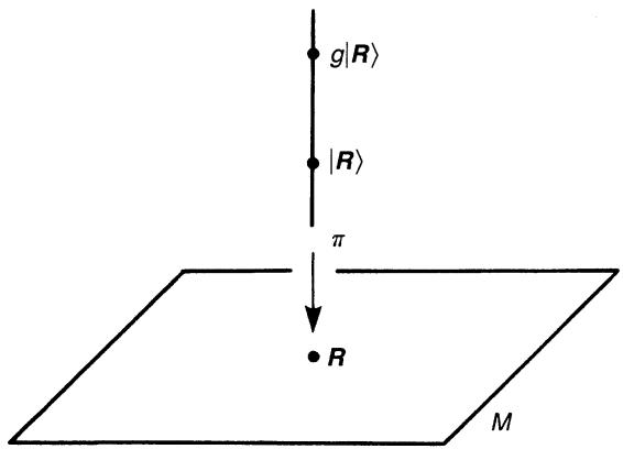
Figure 10.6. The fibre of a quantum mechanical system which depends on adiabatic parameters $\mathbf{R}$ .

Fixing the phase of $|R⟩$ at each point $R\in M$ amounts to choosing a section. Let $\sigma (R)=|R⟩$ be a local section over a chart $U$ of $M$ . The canonical local trivialization is given by

$${\varphi }^{-1}(|\mathbf{R}⟩)=(\mathbf{R},e).\text{\hspace{1em}(10.138)}$$

The ‘right’ action yields

$${\varphi }^{-1}(|\mathbf{R}⟩\cdot g)=(\mathbf{R},e)g=(\mathbf{R},g).\text{\hspace{1em}(10.139)}$$

Now that the bundle structure is defined, we provide it with a connection. Let us define Berry’s connection by

$$\mathcal{A}={\mathcal{A}}_{\mu }\mathrm{d}{R}^{\mu }\equiv ⟨\mathbf{R}|(\mathrm{d}|\mathbf{R})⟩=-(\mathrm{d}⟨\mathbf{R}|)|\mathbf{R}⟩\text{\hspace{1em}(10.140)}$$

where $\mathrm{d}=(\partial /\partial R^{\mu })\mathrm{d}{R}^{\mu }$ is the exterior derivative in $\mathbf{R}$ -space. Note that $\mathcal{A}$ is anti-Hermitian since

$$0=\mathrm{d}(⟨R|R⟩)=(\mathrm{d}⟨R|)|R⟩+⟨R|\mathrm{d}|R⟩=⟨R|\mathrm{d}|R{⟩}^{\ast }+⟨R|\mathrm{d}|R⟩.$$

To see (10.140) is indeed a local form of a connection, we have to check the compatibility condition. Let $U_i$ and $U_j$ be overlapping charts of $M$ and let ${\sigma }_i(\mathbf{R})=|\mathbf{R}{⟩}_i$ and ${\sigma }_j(\mathbf{R})=|\mathbf{R}{⟩}_j$ be the respective local sections. They are related by the transition function as $|\mathbf{R}{⟩}_j=|\mathbf{R}{⟩}_i{t}_{ij}(\mathbf{R})$ . We then find that

$$\begin{array}{rl}{\mathcal{A}}_j(\mathbf{R})& ={\Omega }_j⟨\mathbf{R}|\mathrm{d}|\mathbf{R}{⟩}_j=t_{ij}(\mathbf{R}{)}^{-1}{\Omega }_i⟨\mathbf{R}|[\mathrm{d}|\mathbf{R}{⟩}_i{t}_{ij}(\mathbf{R})+|\mathbf{R}⟩\mathrm{d}{t}_{ij}(\mathbf{R})]\\ & ={\mathcal{A}}_i(\mathbf{R})+t_{ij}(\mathbf{R}{)}^{-1}\mathrm{d}{t}_{ij}(\mathbf{R}).\end{array}\text{\hspace{1em}(10.141)}$$

The set of one-forms $\{{\mathcal{A}}_i\}$ satisfying (10.141) defines an Ehresmann connection on $P(M,\mathrm{U}(1))$ .

The field strength $\mathcal{F}$ of $\mathcal{A}$ is called Berry’s curvature and is given by

$$\mathcal{F}=\mathrm{d}\mathcal{A}=(\mathrm{d}⟨\mathbf{R}|)\wedge (\mathrm{d}|\mathbf{R}⟩)=\left(\frac{\partial ⟨\mathbf{R}|}{\partial R^{\mu }}\right)\left(\frac{\partial |\mathbf{R}⟩}{\partial R^{\nu }}\right)\mathrm{d}{R}^{\mu }\wedge \mathrm{d}{R}^{\nu }.\text{\hspace{1em}(10.142)}$$

After an example from atomic physics, we shall clarify how this geometrical structure is reflected in Berry’s phase.

Example 10.7

Let us consider a quantum mechanical system which contains ‘fast’ degrees of freedom $\mathbf{r}$ and ‘slow’ degrees of freedom $\mathbf{R}$ . For example, we may imagine an electron moving under the potential of slowly vibrating ions. Suppose the Hamiltonian is given by

$$H=\frac{{\mathbf{p}}^2}{2m}+\frac{{\mathbf{P}}^2}{2M}+V(\mathbf{r};\mathbf{R})\text{\hspace{1em}(10.143)}$$

where $p(P)$ is the momentum canonical conjugate to $r(R)$ . As a first approximation, we may consider the slow degrees of freedom are ‘frozen’ at some value $R$ and consider an instantaneous sub-Hamiltonian

$$h(\mathbf{R})=\frac{{\mathbf{p}}^2}{2m}+V(\mathbf{r};\mathbf{R})\text{\hspace{1em}(10.144)}$$

and the eigenvalue problem

$$h(\mathbf{R})|\mathbf{R}⟩={ϵ}_n(\mathbf{R})|\mathbf{R}⟩\text{\hspace{1em}(10.145)}$$

where $|R⟩$ stands for the $n$ th eigenvector $|n;R⟩$ of the ‘fast’ degrees of freedom. We assume that the eigenvalue is isolated and non-degenerate. Berry’s connection is $\mathcal{A}(R)=⟨R|\mathrm{d}|R⟩$ , while the curvature is $\mathcal{F}=(\mathrm{d}⟨R|)\wedge (\mathrm{d}|R⟩)$ .

It is interesting to see how the fast degrees of freedom affect the slow degrees of freedom. We assume the total wavefunction is written in the form

$$\Psi (\mathbf{r};\mathbf{R})=\Phi (\mathbf{R})|\mathbf{R}⟩\text{\hspace{1em}(10.146)}$$

and find the ‘effective’ Schrödinger equation which $\Phi (R)$ , the wavefunction of the ‘slow’ degrees of freedom, satisfies. The eigenvalue problem of the Hamiltonian (10.143) is

$$\begin{array}{rl}& H\Psi (\mathbf{r};\mathbf{R})=-\frac{1}{2M}\left[{\nabla }_{\mathbf{R}}^2\Phi (\mathbf{R})|\mathbf{R}⟩+2{\nabla }_{\mathbf{R}}\Phi (\mathbf{R})\cdot {\nabla }_{\mathbf{R}}|\mathbf{R}⟩+\Phi (\mathbf{R}){\nabla }_{\mathbf{R}}^2|\mathbf{R}⟩\right]\\ & -\Phi (\mathbf{R})\frac{1}{2m}{\nabla }_{\mathbf{r}}^2|\mathbf{R}⟩+\Phi (\mathbf{R})V(\mathbf{r};\mathbf{R})|\mathbf{R}⟩\\ & =E_n(\mathbf{R})\Phi (\mathbf{R})|\mathbf{R}⟩.\end{array}$$

If we multiply $⟨R|$ on the left and use the Schrödinger equation (10.145), this equation becomes

$$\begin{array}{rl}& -\frac{1}{2M}[{\nabla }_{\mathbf{R}}^2\Phi (\mathbf{R})+2{\nabla }_{\mathbf{R}}\Phi (\mathbf{R})\cdot ⟨\mathbf{R}|{\nabla }_{\mathbf{R}}|\mathbf{R}⟩+\Phi (\mathbf{R})\left({⟨\mathbf{R}|{\nabla }_{\mathbf{R}}|\mathbf{R}⟩)}^2\right]\\ & +{ϵ}_n(\mathbf{R})\Phi (\mathbf{R})=E_n(\mathbf{R})\Phi (\mathbf{R})\end{array}\text{\hspace{1em}(10.147)}$$

where we have employed the Born-Oppenheimer approximation, in which all the matrix elements except the diagonal ones are neglected,

$$⟨n;\mathbf{R}|{\nabla }_{\mathbf{R}}|n^{\prime };\mathbf{R}⟩=0n^{\prime }\ne n.\text{\hspace{1em}(10.148)}$$

Now the effective Hamiltonian for $|\Phi (R)⟩$ is given by

$$H_{\text{e f f}}(n)\equiv -\frac{1}{2M}{\left(\frac{\partial }{\partial R^{\mu }}+{\mathcal{A}}_{\mu }(\mathbf{R})\right)}^2+{\epsilon }_n(\mathbf{R})\text{\hspace{1em}(10.149)}$$

where ${\mathcal{A}}_{\mu }$ is a component of Berry’s connection,

$${\mathcal{A}}_{\mu }(\mathbf{R})=⟨\mathbf{R}|\frac{\partial }{\partial {\mathbf{R}}^{\mu }}|\mathbf{R}⟩.\text{\hspace{1em}(10.150)}$$

It is remarkable that the fast degrees of freedom have induced a vector potential coupled to the slow degrees of freedom. Note also that the eigenvalue ${\epsilon }_n(R)$ behaves as a potential energy in $H_{\mathrm{eff}}$ . This ‘spontaneous creation’ of the gauge symmetry reflects the phase degree of freedom of the wavefunction $|R⟩$ .

The Schrödinger equation describing the adiabatic change is

$$H(\mathbf{R}(t))|\mathbf{R}(t),t⟩=\mathrm{i}\frac{\mathrm{d}}{\mathrm{d}t}|\mathbf{R}(t),t⟩\text{\hspace{1em}(10.151a)}$$

where we note that $|R(t),t⟩$ has an explicit $t$ -dependence as well as an implicit one through $R(t)$ . Berry assumes that

$$|\mathbf{R}(t),t⟩=\exp \left(-\mathrm{i}{\int }_0^t{E}_n(t)\mathrm{d}t\right){\mathrm{e}}^{\mathrm{i}\eta (t)}|\mathbf{R}(t)⟩\text{\hspace{1em}(10.152a)}$$

where $|\mathbf{R}⟩$ is an instantaneous normalized eigenstate of $H(\mathbf{R})$ ,

$$\mathcal{H}(\mathbf{R})|\mathbf{R}⟩=E_n(\mathbf{R})|\mathbf{R}⟩⟨\mathbf{R}|\mathbf{R}⟩=1.\text{\hspace{1em}(10.153)}$$

The first exponential is the ordinary dynamical phase while the second one is Berry’s phase. It is convenient for our purpose to define an operator

$$\mathcal{H}(\mathbf{R})\equiv H(\mathbf{R})-E_n(\mathbf{R})\text{\hspace{1em}(10.154)}$$

to dispose of the dynamical phase. The state $|R⟩$ is the zero-energy eigenstate of $\mathcal{H}(R)$ : $\mathcal{H}(R)|R⟩=0$ . The solution of the modified Schrödinger equation,

$$\mathcal{H}(\mathbf{R})|\mathbf{R}(t),t⟩=\mathrm{i}\frac{\mathrm{d}}{\mathrm{d}t}|\mathbf{R}(t),t⟩\text{\hspace{1em}(10.151b)}$$

is then given by

$$|\mathbf{R}(t),t⟩={\mathrm{e}}^{\mathrm{i}\eta (t)}|\mathbf{R}(t)⟩.\text{\hspace{1em}(10.152b)}$$

We found in (10.136) that $\eta$ is given by

$$\eta (t)=\mathrm{i}{\int }_0^t\mathrm{d}s\frac{\mathrm{d}{R}^{\mu }}{\mathrm{d}s}⟨\mathbf{R}(s)|\frac{\partial }{\partial R^{\mu }}|\mathbf{R}(s)⟩=\mathrm{i}{\int }_{\mathbf{R}(0)}^{\mathbf{R}(t)}⟨\mathbf{R}|\mathrm{d}|\mathbf{R}⟩.\text{\hspace{1em}(10.155)}$$

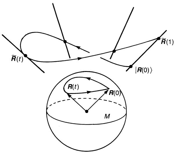
We show that Berry’s phase is a holonomy associated with the connection (10.140) on $P(M,\mathrm{U}(1))$ . Take a section $\sigma (\mathbf{R})=|\mathbf{R}⟩$ over a chart $U$ of $M$ . Let $\mathbf{R}:[0,1]\to M$ be a loop in $U$ .¹ We write a horizontal lift of $\mathbf{R}(t)$ with respect to the connection (10.140) as

$$\tilde{\mathbf{R}}(t)=\sigma (\mathbf{R}(t))g(\mathbf{R}(t))\text{\hspace{1em}(10.156)}$$

where $g(\mathbf{R}(0))$ is taken to be the unit element of $\mathrm{U}(1)$ . The group element $g(t)$ satisfies (10.13b),

$$\frac{\mathrm{d}g(t)}{\mathrm{d}t}g(t{)}^{-1}=-\mathcal{A}\left(\frac{\mathrm{d}}{\mathrm{d}t}\right)=-⟨\mathbf{R}(t)|\frac{\mathrm{d}}{\mathrm{d}t}|\mathbf{R}(t)⟩\text{\hspace{1em}(10.157)}$$

where $g(t)$ stands for $g(R(t))$ . From $g(t)=\exp (\mathrm{i}\eta (t))$ , we obtain

$$\mathrm{i}\frac{\mathrm{d}\eta (t)}{\mathrm{d}t}=-⟨\mathbf{R}(t)|\frac{\mathrm{d}}{\mathrm{d}t}|\mathbf{R}(t)⟩$$

which is easily integrated to yield

$$\eta (1)=\mathrm{i}{\int }_0^1⟨\mathbf{R}(s)|\frac{\mathrm{d}}{\mathrm{d}s}|\mathbf{R}(s)⟩\mathrm{d}s=\mathrm{i}\oint ⟨\mathbf{R}|\mathrm{d}|\mathbf{R}⟩.\text{\hspace{1em}(10.158)}$$

Let us note that $R(0)=R(1)$ , hence $|R(0)⟩=|R(1)⟩$ . Then $\exp [\mathrm{i}\eta (1)]$ is regarded as a holonomy (figure 10.7)

Figure 10.7. If the parameter changes adiabatically along a loop $R(t)$ , the state with initial condition $|R(0)⟩$ becomes $|\tilde{R}(1)⟩$ which is different from $|R(0)⟩$ in general. The difference is the holonomy and is identified with Berry’s phase.

$$\tilde{\mathbf{R}}(1)=\exp \left(-\oint ⟨\mathbf{R}|\mathrm{d}|\mathbf{R}⟩\right)\cdot |\mathbf{R}(0)⟩.\text{\hspace{1em}(10.159a)}$$

Exercise 10.14

Let $S$ be a surface in $M$ , which is bounded by the loop $\mathbf{R}(t)$ . Show that

$$\tilde{\mathbf{R}}(1)=\exp \left(-{\oint }_S\mathcal{F}\right)\cdot |\mathbf{R}(0)⟩\text{\hspace{1em}(10.159b)}$$

where $\mathcal{F}$ is given by (10.142).

Example 10.8

Let us consider a spin- $\frac{1}{2}$ particle in a magnetic field with the Hamiltonian

$$H(\mathbf{R})=\mathbf{R}\cdot \mathbf{\sigma }=\left(\begin{array}{cc}{R}_3& R_1-\mathrm{i}{R}_2\\ R_1+\mathrm{i}{R}_2& -R_3\end{array}\right).\text{\hspace{1em}(10.160)}$$

The parameter $R$ corresponds to the applied magnetic field. This is a two-level system taking eigenvalues $\pm |R|$ . Let us consider the eigenvalue $R=+|R|$ . According to the prescription just described, we introduce a Hamiltonian $\mathcal{H}(R)\equiv H(R)-|R|$ and consider the zero-energy eigenstate of $\mathcal{H}(R)$ given by

$${|\mathbf{R}⟩}_{\mathrm{N}}={\left[2R\left(R+R_3\right)\right]}^{-1/2}\left(\genfrac{}{}{0ex}{}{R+R_3}{R_1+\mathrm{i}{R}_2}\right).\text{\hspace{1em}(10.161)}$$

The gauge potential is obtained after a straightforward but tedious calculation as

$${\mathcal{A}}_{\mathrm{N}}=\mathrm{N}⟨\mathbf{R}|\mathrm{d}|\mathbf{R}{⟩}_{\mathrm{N}}=-\mathrm{i}\frac{R_2\mathrm{d}{R}_1-R_1\mathrm{d}{R}_2}{2R(R+R_3)}.\text{\hspace{1em}(10.162)}$$

The field strength is

$$\mathcal{F}=\mathrm{d}\mathcal{A}=\frac{\mathrm{i}}{2}\frac{R_1\mathrm{d}{R}_2\wedge \mathrm{d}{R}_3+R_2\mathrm{d}{R}_3\wedge \mathrm{d}{R}_1+R_3\mathrm{d}{R}_1\wedge \mathrm{d}{R}_2}{R^3}.\text{\hspace{1em}(10.163)}$$

So far we have assumed that the state $|\mathbf{R}⟩$ is isolated. However, this assumption breaks down if $\mathbf{R}=0$ , in which case two eigenstates are degenerate. Surprisingly, this singularity behaves like a magnetic monopole in $\mathbf{R}$ -space. To see this, we introduce polar coordinates $\theta$ and $\varphi$ in $\mathbf{R}$ -space,

$$R_1=R\sin \theta \cos \varphi R_2=R\sin \theta \sin \varphi R_3=R\cos \theta .$$

The state (10.161) is expressed as

$${|\mathbf{R}⟩}_{\mathrm{N}}=\left(\begin{array}{c}\cos (\theta /2)\\ {\mathrm{e}}^{\mathrm{i}\varphi }\sin (\theta /2)\end{array}\right).\text{\hspace{1em}(10.164)}$$

This state is singular at $\theta =\pi$ , reflecting that $|\mathbf{R}{⟩}_{\mathrm{N}}$ is not defined for $R_3=-R$ . Consider another eigenvector

$$\begin{array}{rl}|\mathbf{R}{⟩}_{\mathrm{S}}\equiv {\mathrm{e}}^{-\mathrm{i}\varphi }|\mathbf{R}{⟩}_{\mathrm{N}}& =\left(\begin{array}{c}{\mathrm{e}}^{-\mathrm{i}\varphi }\cos (\theta /2)\\ \sin (\theta /2)\end{array}\right)\\ & ={\left[2R\left(R-R_3\right)\right]}^{-1/2}\left(\begin{array}{c}{R}_1-\mathrm{i}{R}_2\\ R-R_3\end{array}\right)\end{array}\text{\hspace{1em}(10.165)}$$

with the same eigenvalue. This eigenvector is singular at $\theta =0$ , that is at $R_3=R$ . Corresponding to these vectors, we have Berry’s gauge potentials in polar coordinates,

$${\mathcal{A}}_{\mathrm{N}}=\frac{1}{2}\mathrm{i}(1-\cos \theta )\mathrm{d}\varphi \theta \ne \pi \text{\hspace{1em}(10.166a)}$$

$${\mathcal{A}}_{\mathrm{S}}=-\frac{1}{2}\mathrm{i}(1+\cos \theta )\mathrm{d}\varphi \theta \ne 0.\text{\hspace{1em}(10.166b)}$$

They are related by the gauge transformation,

$${\mathcal{A}}_{\mathrm{S}}={\mathcal{A}}_{\mathrm{N}}-\mathrm{id}\varphi ={\mathcal{A}}_{\mathrm{N}}+{\mathrm{e}}^{\mathrm{i}\varphi }{\mathrm{de}}^{-\mathrm{i}\varphi }\text{\hspace{1em}(10.167)}$$

where $g(\pi /2,\varphi )=\exp (-\mathrm{i}\varphi )$ is identified with the transition function $t_{\mathrm{NS}}$ . Equation (10.166) is simply the vector potential of the Wu-Yang monopole of strength $-\frac{1}{2}$ , see sections 1.9 and 10.5. The total flux of the monopole is $\Phi =4\pi \left(-\frac{1}{2}\right)=-2\pi$ .

The analogy between the present problem and the magnetic monopole is evident by now. If we fix the amplitude $R$ of the magnetic field, the restricted parameter space is $S^2$ . At each point $R$ of $S^2$ , the state has a phase degree of freedom. Thus, we are dealing with a U(1) bundle $P(S^2,\mathrm{U}(1))$ , which also describes a magnetic monopole. For each choice of the parameters $R$ , we have a fibre corresponding to the $n$ th eigenstate $|n;R⟩$ . The fibre at $R$ consists of the equivalence class $[|R⟩]$ defined by (10.137). The projection $\pi$ maps a state to the parameter on which it is defined: $\pi :{\mathrm{e}}^{\mathrm{i}\alpha }|R⟩\to R\in S^2$ . As we have seen, this bundle is non-trivial since it cannot be described by a single connection. The non-triviality of the bundle implies the existence of a monopole at the origin. Note that $R=0$ (that is, $B=0$ ) is a singular point at which all the eigenvalues are degenerate.

Next we turn to the problem of holonomy. Take a standard point $R(0)$ on $S^2$ and choose a vector $|R(0)⟩$ . We choose a loop $R(t)$ on $S^2$ and execute a parallel transportation of $|R(0)⟩$ along $R(t)$ , after which it comes back as a vector $\exp [\mathrm{i}\eta (1)]|R(0)⟩$ . The additional phase $\eta$ represents the holonomy

${\pi }^{-1}(R)\to {\pi }^{-1}(R)$ and corresponds to Berry’s phase. From (10.158), $\eta (1)$ is given by

$$\eta (1)=\mathrm{i}{\oint }_{\mathbf{R}}\mathcal{A}=\mathrm{i}{\int }_S\mathcal{F}\text{\hspace{1em}(10.168)}$$

where $\mathcal{F}=\mathrm{d}\mathcal{A}$ is the field strength and $S$ is the surface bounded by the loop $R(t)$ . It follows from (10.168) that Berry’s phase $\eta (1)$ represents the ‘magnetic flux’ through the area $S$ .

Exercise 10.15

Use (10.165) to show that

$${\mathcal{A}}_{\mathrm{S}}=\frac{\mathrm{i}}{2}\frac{R_2\mathrm{d}{R}_1-R_1\mathrm{d}{R}_2}{R(R-R_3)}.\text{\hspace{1em}(10.169)}$$

Show also that

$$\mathrm{d}\varphi =-\frac{R_2\mathrm{d}{R}_1-R_1\mathrm{d}{R}_2}{(R+R_3)(R-R_3)}.\text{\hspace{1em}(10.170)}$$

Observe that $\mathrm{d}\varphi$ is singular at $R_3=\pm R$ .

10.1 Consider a two-dimensional plane $M$ with coordinate $\mathbf{R}$ and a wavefunction $\psi$ which depends on $\mathbf{R}$ adiabatically as $\psi =\psi (\mathbf{r},\mathbf{R})$ . Let $\mathbf{R}:[0,1]\to M$ be a loop in $M$ and suppose $\psi (r,R(1))=-\psi (r,R(0))$ , that is the phase of $\psi$ changes by $\pi$ after an adiabatic change along the loop. Show that there is a point within the loop at which the adiabatic assumption breaks down. See Longuet-Higgins (1975).

Endnotes

来源与版本

正文：英文 · OCR 机器稿 · 待校对

核对状态：OCR 机器稿 · 待校对

原书 PDF

来源版本：second-edition-local

来源 PDF SHA-256：fcd24c3371d092a8c699ccf5cf0765462924b6c48412804231076e8084b1940d

OCR 来源 SHA-256：0b6324f01172a3548cd34382e82fd8bfae574602b6b2cfaa357ba96bc2c35478

OCR 产物 SHA-256：1742358d726f1864df2d5ab43d3529d419f4e9c7ccc775e50e90f63efa5c2323

Footnotes

1. We shall be a little sloppy in our notation. ↩