12.4 Green’s functions

中文

Distribution theory may often be used to find solutions of inhomogeneous linear partial differential equations by the technique of Green’s functions. We give here two important standard examples.

Poisson’s equation

To solve an inhomogeneous equation such as Poisson’s equation

$${\nabla }^2\varphi =-4\pi \rho \text{\hspace{1em}(12.15)}$$

we seek a solution to the distributional equation

$${\nabla }^{2}G(\mathbf{x}-{\mathbf{x}}^{\prime })={\delta }^3(\mathbf{x}-{\mathbf{x}}^{\prime })=\delta (x-x^{\prime })\delta (y-y^{\prime })\delta (z-z^{\prime }).\text{\hspace{1em}(12.16)}$$

A solution of Poisson’s equation Eq. (12.15) is then

$$\varphi (\mathbf{x})=-\iiint 4\pi \rho ({\mathbf{x}}^{\prime })G(\mathbf{x}-{\mathbf{x}}^{\prime }){\mathrm{d}}^3{x}^{\prime },$$

for

$$\begin{array}{l}{\nabla }^2\varphi =-\iiint 4\pi \rho ({\mathbf{x}}^{\prime }){\nabla }^{2}G(\mathbf{x}-{\mathbf{x}}^{\prime }){\mathrm{d}}^3{x}^{\prime }\\ =-\iiint 4\pi \rho ({\mathbf{x}}^{\prime }){\delta }^3(\mathbf{x}-{\mathbf{x}}^{\prime }){\mathrm{d}}^3{x}^{\prime }\\ =-4\pi \rho (\mathbf{x}).\end{array}$$

To solve, set

$$g(\mathbf{k})=\mathcal{F}G=\frac{1}{(2\pi {)}^{3/2}}{\iiint }_{-\infty }^{\infty }{\mathrm{e}}^{-i\mathbf{k}\cdot \mathbf{y}}G(\mathbf{y}){\mathrm{d}}^{3}y.$$

By Fourier’s theorem

$$G(\mathbf{y})=\frac{1}{(2\pi {)}^{3/2}}{\iiint }_{-\infty }^{\infty }{\mathrm{e}}^{i\mathbf{k}\cdot \mathbf{y}}g(\mathbf{k}){\mathrm{d}}^{3}k,$$

which implies that

$${\nabla }^{2}G(\mathbf{x}-{\mathbf{x}}^{\prime })=\frac{1}{(2\pi {)}^{3/2}}{\iiint }_{-\infty }^{\infty }-{\mathbf{k}}^2{e}^{i\mathbf{k}\cdot (\mathbf{x}-{\mathbf{x}}^{\prime })}g(\mathbf{k})d^{3}k.$$

But

$$\begin{array}{l}\delta (\mathbf{y})=\frac{1}{(2\pi {)}^3}{\int }_{-\infty }^{\infty }{\mathrm{e}}^{i{k}_1{y}_1}\mathrm{d}{k}_1{\int }_{-\infty }^{\infty }{\mathrm{e}}^{i{k}_2{y}_2}\mathrm{d}{k}_2{\int }_{-\infty }^{\infty }{\mathrm{e}}^{i{k}_3{y}_3}\mathrm{d}{k}_3\\ =\frac{1}{(2\pi {)}^3}{\iiint }_{-\infty }^{\infty }{\mathrm{e}}^{i\mathbf{k}\cdot \mathbf{y}}{\mathrm{d}}^{3}k,\end{array}$$

so

$${\delta }^3(\mathbf{x}-{\mathbf{x}}^{\prime })=\frac{1}{2{\pi }^3}{\iiint }_{-\infty }^{\infty }{\mathrm{e}}^{i\mathbf{k}\cdot (\mathbf{x}-{\mathbf{x}}^{\prime })}{\mathrm{d}}^{3}k.$$

Substituting in Eq. (12.16) gives

$$g(\mathbf{k})=-\frac{1}{(2\pi {)}^{3/2}{\mathbf{k}}^2},$$

and

$$G(\mathbf{x}-{\mathbf{x}}^{\prime })=-\frac{1}{(2\pi {)}^3}{\iiint }_{-\infty }^{\infty }\frac{{\mathrm{e}}^{i\mathbf{k}\cdot \mathbf{y}}}{{\mathbf{k}}^2}{\mathrm{d}}^{3}k.\text{\hspace{1em}(12.17)}$$

The integration in $k$-space is best performed using polar coordinates $(k,\theta ,\varphi )$ with the $k_3$ -axis pointing along the direction $\mathbf{R}=\mathbf{x}-{\mathbf{x}}^{\prime }$ (see Fig. 12.2). Then

$$\mathbf{k}\cdot (\mathbf{x}-{\mathbf{x}}^{\prime })=kR\cos \theta (k=\sqrt{\mathbf{k}\cdot \mathbf{k}})$$

and

$${\mathrm{d}}^{3}k=k^2\sin \theta \mathrm{d}k\mathrm{d}\theta \mathrm{d}\varphi .$$

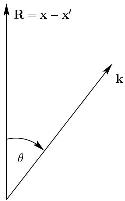Figure 12.2 Change to polar coordinates in $k$-space.

This results in

$$\begin{array}{l}G(\mathbf{R})=-\frac{1}{(2\pi {)}^3}{\int }_0^{\infty }\mathrm{d}k{\int }_0^{\pi }\mathrm{d}\theta {\int }_0^{2\pi }\mathrm{d}\varphi \frac{{\mathrm{e}}^{ikR\cos \theta }}{k^2}{k}^2\sin \theta \\ =-\frac{2\pi }{(2\pi {)}^3}{\int }_0^{\infty }\mathrm{d}k{\int }_0^{\pi }\mathrm{d}\theta \frac{\mathrm{d}}{\mathrm{d}\theta }\left(\frac{-{\mathrm{e}}^{ikR\cos \theta }}{ikR}\right)\\ =-\frac{1}{(2\pi {)}^{2}R}{\int }_0^{\infty }\mathrm{d}k\frac{{\mathrm{e}}^{ikR}-{\mathrm{e}}^{-ikR}}{ik}\\ =-\frac{1}{(2\pi {)}^{2}R}{\int }_0^{\infty }\mathrm{d}k2\frac{\sin kR}{k}\\ =-\frac{1}{4\pi R},\end{array}$$

on making use of the well-known definite integra

$${\int }_0^{\infty }\frac{\sin x}{x}dx=\frac{\pi }{2}.$$

Hence

$$G(\mathbf{x}-{\mathbf{x}}^{\prime })=-\frac{1}{4\pi |\mathbf{x}-{\mathbf{x}}^{\prime }|},\text{\hspace{1em}(12.18)}$$

and a solution of Poisson’s equation Eq. (12.15) is

$$\varphi (\mathbf{x})=\iiint \frac{\rho ({\mathbf{x}}^{\prime })}{|\mathbf{x}-{\mathbf{x}}^{\prime }|}{d}^3{x}^{\prime },$$

where the integral is taken over all of the space, $-\infty <x^{\prime },y^{\prime },z^{\prime }<\infty$ . For a point charge, $\rho (\mathbf{x})=q{\delta }^3(\mathbf{x}-\mathbf{a})$ the solution reduces to the standard coulomb solution

$$\varphi (\mathbf{x})=\frac{q}{|\mathbf{x}-\mathbf{a}|}.$$

Green’s function for the wave equation

To solve the inhomogeneous wave equation

$$\square \psi =-\frac{{\partial }^2}{c^2\partial t^2}\psi +{\nabla }^2\psi =f(\mathbf{x},t)\text{\hspace{1em}(12.19)}$$

it is best to adopt a relativistic 4-vector notation, setting $x^4=ct$ . The wave equation can then be written as in Section 9.4,

$$\square \psi =g^{\mu \nu }\frac{\partial }{\partial x^{\mu }}\frac{\partial }{\partial x^{\nu }}\psi =f(x)$$

where $\mu$ and $\nu$ range from 1 to $4$, $g^{\mu \nu }$ is the diagonal metric tensor having diagonal components $1,1,1,-1$ and the argument $x$ in the last term is shorthand for $(\mathbf{x},x^4)$ ).

Again we look for a solution of the equation

$$\square G(x-x^{\prime })={\delta }^4(x-x^{\prime })\equiv \delta (x^1-x^{\prime 1})\delta (x^2-x^{\prime 2})\delta (x^3-x^{\prime 3})\delta (x^4-x^{\prime 4}).\text{\hspace{1em}(12.20)}$$

Every Green’s function $G$ generates a solution ${\psi }_G(x)$ of Eq. (12.19),

$${\psi }_G(x)=\iiint \int G(x-x^{\prime })f(x^{\prime }){\mathrm{d}}^4{x}^{\prime }$$

for

$$\square {\psi }_G=\iiint \square G(x-x^{\prime })f(x^{\prime }){\mathrm{d}}^4{x}^{\prime }=\iiint {\delta }^4(x-x^{\prime })f(x^{\prime }){\mathrm{d}}^4{x}^{\prime }=f(x).$$

Exercise

Show that the general solution of the inhomogeneous wave equation Eq. (12.19) has the form ${\psi }_G(x)+\varphi (x)$ where $\sqcap \varphi =0$

Set

$$G(x-x^{\prime })=\frac{1}{(2\pi {)}^2}\iiint \int g(k)e^{ik.(x-x^{\prime })}{d}^{4}k$$

where $k=(k_1,k_2,k_3,k_4)$ , and

$$k.(x-x^{\prime })=k_{\mu }(x^{\mu }-x^{\prime \mu })=k_4(x^4-x^{\prime 4})+\mathbf{k}.\cdot (\mathbf{x}-{\mathbf{x}}^{\prime })$$

and ${\mathrm{d}}^{4}k=\mathrm{d}{k}_1\mathrm{d}{k}_2\mathrm{d}{k}_3\mathrm{d}{k}_4$ . Writing the four-dimensional $\delta$ function as a Fourier transform we have

$$\begin{array}{c}\square G(x-x^{\prime })=\frac{1}{(2\pi {)}^2}\iiint \iint -k^{2}g(k){\mathrm{e}}^{ik.(x-x^{\prime })}{\mathrm{d}}^{4}k\\ ={\delta }^4(x-x^{\prime })=\frac{1}{(2\pi {)}^4}\iiint \iint e^{ik.(x-x^{\prime })}{\mathrm{d}}^{4}k,\end{array}$$

whence

$$g(k)=-\frac{1}{4{\pi }^2{k}^2}$$

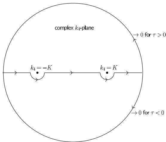Figure 12.3 Green’s function for the three-dimensional wave equation

where $k^2\equiv k.k=k_{\mu }{k}^{\mu }$ . The Fourier transform expression of the Green’s function is thus

$$G(x-x^{\prime })=-\frac{1}{(2\pi {)}^4}\iiint \int \frac{{\mathrm{e}}^{ik.(x-x^{\prime })}}{k^2}{\mathrm{d}}^{4}k.\text{\hspace{1em}(12.21)}$$

To evaluate this integral set

$$\tau =x^4-{x^{\prime }}^4,\mathbf{R}=\mathbf{x}-{\mathbf{x}}^{\prime },K=|\mathbf{k}|=\sqrt{\mathbf{k}\cdot \mathbf{k}},$$

whence $k^2=K^2-k_4^2$ and

$$G(x-x^{\prime })=\frac{1}{(2\pi {)}^4}{\int }_{-\infty }^{\infty }\mathrm{d}{k}_4\frac{{\mathrm{e}}^{i{k}_4\tau }}{k_4^2-K^2}\iiint {\mathrm{d}}^{3}k{\mathrm{e}}^{i\mathbf{k}\cdot \mathbf{R}}.$$

Deform the path in the complex $k_4-\mathrm{plane}$ to avoid the pole singularities at $k_4=\pm K$ as shown in Fig. 12.3 – convince yourself, however, that this has no effect on $G$ satisfying Eq. (12.20).

For $\tau >0$ the contour is completed in a counterclockwise sense by the upper half semi circle and

$$\begin{array}{c}{\int }_{-\infty }^{\infty }\frac{{\mathrm{e}}^{i{k}_4\tau }}{k_4^2-K^2}\mathrm{d}{k}_4=2\pi i\times \text{ sum of residues }\\ =2\pi i(\frac{{\mathrm{e}}^{iK\tau }}{2K}-\frac{{\mathrm{e}}^{-iK\tau }}{2K}).\end{array}$$

For $\tau <0$ we complete the contour with the lower semicircle in a clockwise direction; no poles are enclosed and the integral vanishes. Hence

$${\int }_{-\infty }^{\infty }\frac{{\mathrm{e}}^{i{k}_4\tau }}{k_4^2-K^2}\mathrm{d}{k}_4=-\frac{2\pi }{K}\theta (\tau )\sin K\tau$$

where $\theta (\tau )$ is the Heaviside step function.

This particular contour gives rise to a Green’s function that vanishes for $\tau <0;$ ; that is, for $x^4<x^{\prime 4}$ . It is therefore called the outgoing wave condition or retarded Green’s function, for a source switched on at $({\mathbf{X}}^{\prime },x^{\prime 4})$ only affects field points at later times. Ifthe contour had been chosen to lie above the poles, then the ingoing wave condition or advanced Green’s function would have resulted.

To complete the calculation of $G$ , use polar coodinates in $k$-space with the $k$ -axis paralle to $\mathbb{R}$. This gives

$$\begin{array}{l}G(x-x^{\prime })=-\frac{1}{(2\pi {)}^3}\theta (\tau ){\int }_0^{2\pi }\mathrm{d}\varphi {\int }_0^{\infty }\mathrm{d}K{\int }_0^{\pi }\mathrm{d}\theta K^2\sin \theta {\mathrm{e}}^{iKR\cos \theta }\frac{\sin K\tau }{K}\\ =-\frac{\theta (\tau )}{2{\pi }^{2}R}{\int }_0^{\infty }\mathrm{d}K\sin K\tau \sin KR\\ =-\frac{\theta (\tau )}{2{\pi }^{2}R}{\int }_0^{\infty }\mathrm{d}K\frac{({\mathrm{e}}^{iK\tau }-{\mathrm{e}}^{-iK\tau })}{2i}\frac{({\mathrm{e}}^{iKR}-{\mathrm{e}}^{-iKR})}{2i}\\ =\frac{\theta (\tau )}{4\pi R}(\delta (\tau +R)-\delta (\tau -R))\\ =-\frac{\delta (\tau -R)}{4\pi R}.\end{array}$$

The last step follows because the whole expression vanishes for $\tau <0$ on account of the $\theta (\tau )$ factor, while for $\tau >0$ we have $\delta (\tau +R)=0$ . Hence the Green’s function may be written

$$G(x-x^{\prime })=-\frac{1}{4\pi |\mathbf{x}-{\mathbf{x}}^{\prime }|}\delta (x^4-x^{\prime 4}-|\mathbf{x}-{\mathbf{x}}^{\prime }|),\text{\hspace{1em}(12.22)}$$

which is non-vanishing only on the future light cone of $x^{\prime }$

The solution of the inhomogeneous wave equation Eq. (12.19) generated by this Green’s function is

$$\begin{array}{rl}\psi (\mathbf{x},t)& =\iiint G(x-x^{\prime })f(x^{\prime }){\mathrm{d}}^4{x}^{\prime }\\ & =-\frac{1}{4\pi }\iiint \frac{[f({\mathbf{x}}^{\prime },t^{\prime }){]}_{\text{ ret }}}{|\mathbf{x}-{\mathbf{x}}^{\prime }|}{\mathrm{d}}^3{x}^{\prime }\end{array}\text{\hspace{1em}(12.23)}$$

where $[f({\mathbf{x}}^{\prime },t^{\prime }){]}_{\mathrm{ret}}$ means $f$ evaluated at the retarded time

$$t^{\prime }=t-\frac{|\mathbf{x}-{\mathbf{x}}^{\prime }|}{c}.$$

Problems

Problem 12.15

Show that the Green’s function for the time-independent Klein–Gordon equation

$$({\nabla }^2-m^2)\varphi =\rho (\mathbf{r})$$

can be expressed as the Fourier integra

$$G(\mathbf{x}-{\mathbf{x}}^{\prime })=-\frac{1}{(2\pi {)}^3}\int \int \int {\mathrm{d}}^{3}k\frac{{\mathrm{e}}^{i\mathbf{k}.(\mathbf{x}-{\mathbf{x}}^{\prime })}}{{\mathbf{k}}^2+m^2}.$$

Evaluate this integral and show that it results in

$$G(\mathbf{R})=-\frac{{\mathrm{e}}^{-mR}}{4\pi R}\text{ where }\mathbf{R}=\mathbf{x}-{\mathbf{x}}^{\prime },R=|\mathbf{R}|.$$

Find the solution $\varphi$ corresponding to a point source

$$\rho (\mathbf{r})=q{\delta }^3(\mathbf{r}).$$

Problem 12.16

Show that the Green’s function for the one-dimensional diffusion equation,

$$\frac{{\partial }^{2}G(x,t)}{\partial x^2}-\frac{1}{\kappa }\frac{\partial G(x,t)}{\partial t}=\delta (x-x^{\prime })\delta (t-t^{\prime })$$

is given by

$$G(x-x^{\prime },t-t^{\prime })=-\theta (t-t^{\prime })\sqrt{\frac{\kappa }{4\pi (t-t^{\prime })}}{\mathrm{e}}^{-(x-x^{\prime }{)}^2/4\kappa (t-t^{\prime })},$$

and write out the corresponding solution of the inhomogeneous equation

$$\frac{{\partial }^2\psi (x,t)}{\partial x^2}-\frac{1}{\kappa }\frac{\partial \psi (x,t)}{\partial t}=F(x,t).$$

Do the same for the two- and three-dimensional diffusion equations

$${\nabla }^{2}G(x,t)-\frac{1}{\kappa }\frac{\partial G(x,t)}{\partial t}={\delta }^n(\mathbf{x}-{\mathbf{x}}^{\prime })\delta (t-t^{\prime })(n=2,3).$$