2.1 Manifolds

The stage on which our story will play out is a mathematical object called a manifold. We will give a precise definition below, but for now you should think of a manifold as a curved, n-dimensional space. If you zoom in to any patch, the manifold looks like ${\mathbf{R}}^n$ But, viewed more globally, the manifold may have interesting curvature or topology.

To begin with, our manifold will have very little structure. For example, initially there will be no way to measure distances between points. But as we proceed, we will describe the various kinds of mathematical objects that can be associated to a manifold, and each one will allow us to do more and more things. It will be a surprisingly long time before we can measure distances between points! (Not until Section 3.)

You have met many manifolds in your education to date, even if you didn’t call them by name. Some simple examples in mathematics include Euclidean space ${\mathbf{R}}^n$ the sphere ${\mathbf{S}}^n$ , and the torus ${\mathbf{T}}^n={\mathbf{S}}^1\times \dots \times {\mathbf{S}}^1$ . Some simple examples in physics include the configuration space and phase space that we use in classical mechanics and the state space of thermodynamics. As we progress, we will see how familiar ideas in these subjects can be expressed in a more formal language. Ultimately our goal is to explain how spacetime is a manifold and to understand the structures that live on it.

2.1.1 Topological Spaces

Even before we get to a manifold, there is some work to do in order to define the underlying object. What follows is the mathematical equivalent of reading a biography about an interesting person and having to spend the first 20 pages wading through a description of what their grandparents did for a living. This backstory will not be particularly useful for our needs and we include it here only for completeness. We’ll keep it down to one page.

Our backstory is called a topological space. Roughly speaking, this is a space in which each point can be viewed as living in a neighbourhood of other points, in a manner that allows us to define concepts such as continuity and convergence.

Definition

A topological space M is a set of points, endowed with a topology T . This is a collection of open subsets $\{{\mathcal{O}}_{\alpha }\subset M\}$ which obey:

i) Both the set M and the empty set ∅ are open subsets: $M\in \tau$ and $\varnothing \in \mathcal{T}$

ii) The intersection of a finite number of open sets is also an open set. So if ${\mathcal{O}}_1\in \mathcal{T}$ and ${\mathcal{O}}_2\in \mathcal{T}$ then ${\mathcal{O}}_1\cap {\mathcal{O}}_2\in \mathcal{T}$

iii) The union of any number (possibly infinite) of open sets is also an open set. So if ${\mathcal{O}}_{\gamma }\in \mathcal{T}$ then ${\cup }_{\gamma }{\mathcal{O}}_{\gamma }\in \mathcal{T}$

Given a point $p\in M$ , we say that $\mathcal{O}\in \mathcal{T}$ is a neighbourhood of p if $p\in \mathcal{O}$ . This concept leads us to our final requirement: we require that, given any two distinct points, there is a neighbourhood which contains one but not the other. In other words, for any $p,q\in M$ with $p\ne q$ , there exists ${\mathcal{O}}_1,{\mathcal{O}}_2\in \mathcal{T}$ such that $p\in {\mathcal{O}}_1$ and $q\in {\mathcal{O}}_2$ and ${\mathcal{O}}_1\cap {\mathcal{O}}_2=\varnothing$ . Topological spaces which obey this criterion are called Hausdorff. It is like a magic ward to protect us against bad things happening.

An example of a good Hausdorff space is the real line, $M=\mathbf{R}$ , with T consisting of all open intervals $(a,b)$ , with $a<b\in \mathbf{R}$ , and their unions. An example of a non-Hausdorff space is any M with $\mathcal{T}=\{M,\varnothing \}$

Definition

One further definition (it won’t be our last). A homeomorphism between topological spaces $(M,\tau )$ and $(\tilde{M},\tilde{\tau })$ is a map $f:M\to \tilde{M}$ which is

i) Injective (or one-to-one): for $p\ne q,f(p)\ne f(q)$

ii) Surjective (or onto): $f(M)=\tilde{M}$ , which means that for each $\tilde{p}\in \tilde{M}$ there exists a $p\in M$ such that $f(\mathbf{p})=\tilde{\mathbf{p}}.$

Functions which are both injective and surjective are said to be bijective. This ensures that they have an inverse

iii) Bicontinuous. This means that both the function and its inverse are continuous. To define a notion of continuity, we need to use the topology. We say that $f$ is continuous if, for all $\tilde{\mathcal{O}}\in \tilde{\mathcal{T}},f^{-1}(\tilde{\mathcal{O}})\in \mathcal{T}$

There’s an animation of a donut morphing into a coffee mug and back that is often used to illustrate the idea of topology. If you want to be fancy, you can say that a donut is homeomorphic to a coffee mug.

2.1.2 Differentiable Manifolds

We now come to our main character: an n-dimensional manifold is a space which, locally, looks like ${\mathbf{R}}^n$ . Globally, the manifold may be more interesting than ${\mathbf{R}}^n$ , but the idea is that we can patch together these local descriptions to get an understanding for the entire space.

Definition

An n-dimensional differentiable manifold is a Hausdorff topological space M such that

i) M is locally homeomorphic to ${\mathbf{R}}^n$ . This means that for each $p\in M$ , there is an open set $\mathcal{O}$ such that $p\in \mathcal{O}$ and a homeomorphism $\varphi :\mathcal{O}\to U$ with $U$ an open subset of ${\mathbf{R}}^n$

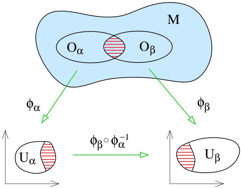
ii) Take two open subsets ${\mathcal{O}}_{\alpha }$ and ${\mathcal{O}}_{\beta }$ that overlap, so that ${\mathcal{O}}_{\alpha }\cap {\mathcal{O}}_{\beta }\ne \varnothing$ . We require that the corresponding maps ${\varphi }_{\alpha }:{\mathcal{O}}_{\alpha }\to U_{\alpha }$ and ${\varphi }_{\beta }:{\mathcal{O}}_{\beta }\to U_{\beta }$ are compatible, meaning that the map ${\varphi }_{\beta }\circ {\varphi }_{\alpha }^{-1}:{\varphi }_{\alpha }({\mathcal{O}}_{\alpha }\cap {\mathcal{O}}_{\beta })\to {\varphi }_{\beta }({\mathcal{O}}_{\alpha }\cap {\mathcal{O}}_{\beta })$ is smooth (also known as infinitely differentiable or $C^{\infty })$ , as is its inverse. This is depicted in Figure 10.

The maps ${\varphi }_{\alpha }$ are called charts and the collection of charts is called an atlas. You should think of each chart as providing a coordinate system to label the region ${\mathcal{O}}_{\alpha }$ of $M.$ . The coordinate associated to $p\in {\mathcal{O}}_{\alpha }$ is

$${\varphi }_{\alpha }(p)=\left(x^1(p),\dots ,x^n(p)\right)$$

We write the coordinate in shorthand as simply $x^{\mu }(p)$ , with $\mu =1,\dots ,n$ . Note that we use a superscript $\mu$ rather than a subscript: this simple choice of notation will prove useful as we go along.

Figure 10. Charts on a manifold.

If a point p is a member of more than one subset O then it may have a number of different coordinates associated to it. There’s nothing to be nervous about here: it’s entirely analogous to labelling a point using either Euclidean coordinate or polar coordinates.

The maps ${\varphi }_{\beta }\circ {\varphi }_{\alpha }^{-1}$ take us between different coordinate systems and are called transition functions. The compatibility condition is there to ensure that there is no inconsistency between these different coordinate systems.

Any manifold M admits many different atlases. In particular, nothing stops us from adding another chart to the atlas, provided that it is compatible with all the others. Two atlases are said to be compatible if every chart in one is compatible with every chart in the other. In this case, we say that the two atlases define the same differentiable structure on the manifold.

Examples

Here are a few simple examples of differentiable manifolds:

• $R^n$: this looks locally like ${\mathbf{R}}^n$ because it is $R^n$. You only need a single chart with the usual Euclidean coordinates. Similarly, any open subset of ${\mathbf{R}}^n$ is a manifold.

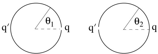
Figure 11. Two charts on a circle. The figures are subtly different! On the left, point $q$ is removed and ${\theta }_1\in (0,2\pi )$ . On the right, point $q^{\prime }$ is removed and ${\theta }_2\in (-\pi ,\pi )$

${\mathbf{S}}^1$ : The circle can be defined as a curve in ${\mathbf{R}}^2$ with coordinates (cos θ, sin θ). Until now in our physics careers, we’ve been perfectly happy taking $\theta \in [0,2\pi )$ as the coordinate on ${\mathbf{S}}^1$ . But this coordinate does not meet our requirements to be a chart because it is not an open set. This causes problems if we want to differentiate functions at $\theta =0:$ to do so we need to take limits from both sides but there is no coordinate with θ a little less than zero.

To circumvent this, we need to use at least two charts to cover ${\mathbf{S}}^1$ . For example, we could pick out two antipodal points, say $q=(1,0)$ and $q^{\prime }=(-1,0)$ . We take the first chart to cover ${\mathcal{O}}_1={\mathbf{S}}^1-\{q\}$ with the map ${\varphi }_1:{\mathcal{O}}_1\to (0,2\pi )$ defined by ${\varphi }_1(p)=\theta$ as shown in the left-hand of Figure 11. We take the second chart to cover ${\mathcal{O}}_2={\mathbf{S}}^1-\{q^{\prime }\}$ with the map ${\varphi }_2:{\mathcal{O}}_2\to (-\pi ,\pi )$ defined by ${\varphi }_2(p)={\theta }^{\prime }$ as shown in the right-hand figure.

The two charts overlap on the upper and lower semicircles. The transition function is given by

$${\theta }^{\prime }={\varphi }_2({\varphi }_1^{-1}(\theta ))=\{\begin{array}{cl}\theta & \text{ if }\theta \in (0,\pi )\\ \theta -2\pi & \text{ if }\theta \in (\pi ,2\pi )\end{array}$$

The transition function isn’t defined at $\theta =0$ , corresponding to the point $q_1$ , nor at $\theta =\pi$ , corresponding to the point $q_2$ . Nonetheless, it is smooth on each of the two open intervals as required.

${\mathbf{S}}^2;$ It will be useful to think of the sphere as the surface $x^2+y^2+z^2=1$ embedded in Euclidean ${\mathbf{R}}^3$ . The familiar coordinates on the sphere ${\mathbf{S}}^2$ are those inherited from spherical polar coordinates of ${\mathbf{R}}^3$ , namely

$$x=\sin \theta \cos \varphi ,y=\sin \theta \sin \varphi ,z=\cos \theta \text{\hspace{1em}(2.1)}$$

with $\theta \in [0,\pi ]$ and $\varphi \in [0,2\pi )$ . But as with the circle ${\mathbf{S}}^1$ described above, these are not open sets so will not do for our purpose. In fact, there are two distinct issues. If we focus on the equator at $\theta =\pi /2$ , then the coordinate $\varphi \in [0,2\pi )$ parameterises a circle and suffers the same problem that we saw above. On top of this, at the north pole $\theta =0$ and south pole $\theta =\pi$ , the coordinate $\varphi$ is not well defined, since the value of $\theta$ has already specified the point uniquely. This manifests itself on Earth by the fact that all time zones coincide at the North pole. It’s one of the reasons people don’t have business meetings there.

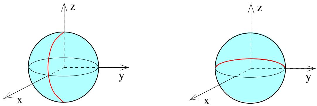
Figure 12. Two charts on a sphere. In the left-hand figure, we have removed the half-equator defined as $y=0$ with $x>0$ , shown in red. In right-figure, we have removed the half-equator $z=0$ with $x<0$ , again shown in red.

Once again, we can resolve these issues by introducing two charts covering different patches on ${\mathbf{S}}^2$ . The first chart applies to the sphere ${\mathbf{S}}^2$ with a line of longitude removed, defined by $y=0$ and $x>0$ , as shown in Figure 12. (Think of this as the dateline.) This means that neither the north nor south pole are included in the open set ${\mathcal{O}}_1$ . On this open set, we define a map ${\varphi }_1:{\mathcal{O}}_1\to {\mathbf{R}}^2$ using the coordinates (2.1), now with $\theta \in (0,\pi )$ and $\varphi \in (0,2\pi )$ , so that we have a map to an open subset of ${\mathbf{R}}^2$

We then define a second chart on a different open set ${\mathcal{O}}_2$ , defined by ${\mathbf{S}}^2$ , with the line $z=0$ and $x<0$ removed. Here we define the map ${\varphi }_2:{\mathcal{O}}_2\to {\mathbf{R}}^2$ using the coordinates

$$x=-\sin {\theta }^{\prime }\cos {\varphi }^{\prime },y=\cos {\theta }^{\prime },z=\sin {\theta }^{\prime }\sin {\varphi }^{\prime }$$

with ${\theta }^{\prime }\in (0,\pi )$ and $\varphi \in (0,2\pi )$ . Again this is a map to an open subset of ${\mathbf{R}}^2$ . We have ${\mathcal{O}}_1\cup {\mathcal{O}}_2={\mathbf{S}}^2$ while, on the overlap ${\mathcal{O}}_1\cap {\mathcal{O}}_2$ , the transition functions ${\varphi }_1\circ {\varphi }_2^{-1}$ 1 and ${\varphi }_2\circ {\varphi }_1^{-1}$ are smooth. (We haven’t written these functions down explicitly, but it’s clear that they are built from cos and sin functions acting on domains where their inverses exist.)

Note that for both ${\mathbf{S}}^1$ and ${\mathbf{S}}^2$ examples above, we made use of the fact that they can be viewed as embedded in a higher dimensional ${\mathbf{R}}^{n+1}$ to construct the charts. However, this isn’t necessary. The definition of a manifold makes no mention of a higher dimensional embedding and these manifolds should be viewed as having an existence independent of any embedding.

As you can see, there is a level of pedantry involved in describing these charts. (Mathematicians prefer the word “rigour”.) The need to deal with multiple charts arises only when we have manifolds of non-trivial topology; the manifolds ${\mathbf{S}}^1$ and ${\mathbf{S}}^2$ that we met above are particularly simple examples. When we come to discuss general relativity, we will care a lot about changing coordinates, and the limitations of certain coordinate systems, but our manifolds will turn out to be simple enough that, for all practical purposes, we can always find a single set of coordinates that tells us what we need to know. However, as we progress in physics, and topology becomes more important, so too does the idea of different charts. Perhaps the first place in physics where overlapping charts become an integral part of the discussion is the construction of a magnetic monopole. (See the lectures on Gauge Theory.)

2.1.3 Maps Between Manifolds

The advantage of locally mapping a manifold to ${\mathbf{R}}^n$ is that we can now import our knowledge of how to do maths on ${\mathbf{R}}^n$ . For example, we know how to differentiate functions on ${\mathbf{R}}^n$ , and what it means for functions to be smooth. This now translates directly into properties of functions defined over the manifold.

We say that a function $f:M\to \mathbf{R}$ is smooth, if the map $f\circ {\varphi }^{-1}:U\to \mathbf{R}$ is smooth for all charts $\varphi .$

Similarly, we say that a map $f:M\to N$ between two manifolds M and N (which may have different dimensions) is smooth if the map ψ ◦ $f\circ {\varphi }^{-1}:U\to V$ is smooth for all charts $\varphi :M\to U\subset {\mathbf{R}}^{\dim (M)}$ and $\psi :N\to V\subset {\mathbf{R}}^{\dim (N)}$

A diffeomorphism is defined to be a smooth homeomorphism $f:M\to N$ . In other words it is an invertible, smooth map between manifolds M and N that has a smooth inverse. If such a diffeomorphism exists then the manifolds M and N are said to be diffeomorphic. The existence of an inverse means M and N necessarily have the same dimension.

Manifolds which are homeomorphic can be continuously deformed into each other. But diffeomorphism is stronger: it requires that the map and its inverse are smooth. This gives rise to some curiosities. For example, it turns out that the sphere ${\mathbf{S}}^7$ can be covered by a number of different, incompatible atlases. The resulting manifolds are homeomorphic but not diffeomorphic. These are referred to as exotic spheres. Similarly, Euclidean space ${\mathbf{R}}^n$ has a unique differentiable structure, except for ${\mathbf{R}}^4$ where there are an infinite number of inequivalent structures. I know of only one application of exotic spheres to physics (a subtle global gravitational anomaly in superstring theory) and I know of no applications of the exotic differential structure on ${\mathbf{R}}^4$ . Certainly these will not play any role in these lectures.

来源与版本

正文：英文 · OCR 机器稿 · 待校对

核对状态：OCR 机器稿 · 待校对

原书 PDF

来源版本：michaelmas-2019-source-20260923

来源 PDF SHA-256：3ba65dc61f22a69c7d5fdf3e8e1f641efbfa6cf49a44b3dcb0fd5367ba9fcf1c

OCR 来源 SHA-256：f58e775c8ca9f14ce79c624d8e60dcf8f6b8feacb94e5342e9bfd0dc174328a5

OCR 产物 SHA-256：c1d26eb0446b267ad7684d77fcef336d963e362b9875435f968ce96d8e062d48