2.2 Tangent Spaces

Our next task is to understand how to do calculus on manifolds. We start here with differentiation; it will take us a while longer to get to integration, which we will finally meet in Section 2.4.4.

Consider a function $f:M\to \mathbf{R}$ . To differentiate the function at some point $p,$ we introduce a chart $\varphi =(x^1,\dots ,x^n)$ in a neighbourhood of $p.$ We can then construct the map $f\circ {\varphi }^{-1}:U\to \mathbf{R}$ with $U\subset {\mathbf{R}}^n$ . But we know how to differentiate functions on ${\mathbf{R}}^n$ and this gives us a way to differentiate functions on $M$ , namely

$${\frac{\partial f}{\partial x^{\mu }}|}_p:={\frac{\partial (f\circ {\varphi }^{-1})}{\partial x^{\mu }}|}_{\varphi (p)}\text{\hspace{1em}(2.2)}$$

Clearly this depends on the choice of chart $\varphi$ and coordinates $x^{\mu }$ . We would like to give a coordinate independent definition of differentiation, and then understand what happens when we choose to describe this object using different coordinates.

2.2.1 Tangent Vectors

We will consider smooth functions over a manifold M. We denote the set of all smooth functions as $C^{\infty }(M)$ .

Definition

A tangent vector $X_p$ is an object that differentiates functions at a point $p\in M$ . Specifically, $X_p:C^{\infty }(M)\to \mathbf{R}$ satisfying

i) Linearity: $X_p(f+g)=X_p(f)+X_p(g)$ for all $f,g\in C^{\infty }(M)$

ii) $X_p(f)=0$ when $f$ is the constant function.

iii) Leibnizarity: $X_p(fg)=f(p)X_p(g)+X_p(f)g(p)$ for all $f,g\in C^{\infty }(M)$ . This, of course, is the product rule.

Note that ii) and iii) combine to tell us that $X_p(af)=a{X}_p(f)$ for $a\in \mathbf{R}$

This definition is one of the early surprises in differential geometry. The surprise is really in the name “tangent vector”. We know what vectors are from undergraduate physics, and we know what differential operators are. But we’re not used to equating the two. Before we move on, it might be useful to think about how this definition fits with other notions of vectors that we’ve met before.

The first time we meet a vector in physics is usually in the context of Newtonian mechanics, where we describe the position of a particle as a vector x in ${\mathbf{R}}^3$ . This concept of a vector is special to flat space and does not generalise to other manifolds. For example, a line connecting two points on a sphere is not a vector and, in general, there is no way to think of a point $p\in M$ as a vector. So we should simply forget that points in ${\mathbf{R}}^3$ can be thought of as vectors.

The next type of vector is the velocity of a particle, $\mathbf{v}=\dot{\mathbf{x}}$ . This is more pertinent. It clearly involves differentiation and, moreover, is tangent to the curve traced out by the particle. As we will see below, velocities of particles are indeed examples of tangent vectors in differential geometry. More generally, tangent vectors tell us how things change in a given direction. They do this by differentiating.

It is simple to check that the object

$${{\partial }_{\mu }|}_p:={\frac{\partial }{\partial x^{\mu }}|}_p$$

which acts on functions as shown in (2.2) obeys all the requirements of a tangent vector.

Note that the index $\mu$ is now a subscript, rather than superscript that we used for the coordinates $x^{\mu }$ . (On the right-hand-side, the superscript in $\partial /\partial x^{\mu }$ is in the denominator and counts as a subscript.) We will adopt the summation convention, where repeated indices are summed. But, as we will see, the placement of indices up or down will tell us something and all sums will necessarily have one index up and one index down. This is a convention that we met already in Special Relativity where the up/downness of the index changes minus signs. Here it has a more important role that we will see as we go on: the placement of the index tells us what kind of mathematical space the object lives in. For now, you should be aware that any equation with two repeated indices that are both up or both down is necessarily wrong, just as any equation with three or more repeated indices is wrong.

Theorem

The set of all tangent vectors at point $p$ forms an $n\cdot$ -dimensional vector space. We call this the tangent space $T_p(M)$ . The tangent vectors ${\partial }_{\mu }{|}_p$ provide a basis for $T_p(M)$ . This means that we can write any tangent vector as

$$X_p=X^{\mu }{{\partial }_{\mu }|}_p$$

with $X^{\mu }=X_p(x^{\mu })$ the components of the tangent vector in this basis.

Proof

Much of the proof is just getting straight what objects live in what spaces. Indeed, getting this straight is a large part of the subject of differential geometry. To start, we need a small lemma. We define the function $F=f\circ {\varphi }^{-1}:U\to \mathbf{R}$ , with $\varphi =(x^1,\dots ,x^n)$ a chart on a neighbourhood of $p.$ Then, in some (perhaps smaller) neighbourhood of p we can always write the function F as

$$F(x)=F(x^{\mu }(p))+(x^{\mu }-x^{\mu }(p))F_{\mu }(x)\text{\hspace{1em}(2.3)}$$

where we have introduced n new functions $F_{\mu }(x)$ and used the summation convention in the final term. If the function F has a Taylor expansion then we can trivially write it in the form (2.3) by repackaging all the terms that are quadratic and higher into the $F_{\mu }(x)$ functions, keeping a linear term out front. But in fact there’s no need to assume the existence of a Taylor expansion. One way to see this is to note that for any function $G(t)$ we trivially have $\begin{array}{r}G(1)=G(0)+{\int }_0^{1}dt{G}^{\prime }(t)\end{array}$ . But now apply this formula to the function $G(t)=F(tx)$ for some fixed x. This gives $\begin{array}{r}F(x)=F(0)+x{\int }_0^{1}dt{F}^{\prime }(xt)\end{array}$ which is precisely (2.3) for a function of a single variable expanded about the origin. The same method holds more generally.

Given (2.3), we act with ${\partial }_{\mu }$ on both sides, and then evaluate at $x^{\mu }=x^{\mu }(p)$ . This tells us that the functions $F_{\mu }$ must satisfy

$${\frac{\partial F}{\partial x^{\mu }}|}_{x(p)}=F_{\mu }(x(p))\text{\hspace{1em}(2.4)}$$

We can translate this into a similar expression for f itself. We define n functions on M by $f_{\mu }=F_{\mu }\circ \varphi$ . Then, for any $q\in M$ in the appropriate neighbourhood of $p,$ (2.3) becomes

$$f\circ {\varphi }^{-1}(x^{\mu }(q))=f\circ {\varphi }^{-1}(x^{\mu }(p))+(x^{\mu }(q)-x^{\mu }(p))[f_{\mu }\circ {\varphi }^{-1}(x^{\mu }(q))]$$

But ${\varphi }^{-1}(x^{\mu }(q))=q$ . So we find that, in the neighbourhood of $p_{:}$ , it is always possible to write a function f as

$$f(q)=f(p)+\left(x^{\mu }(q)-x^{\mu }(p)\right)f_{\mu }(q)$$

for some $f_{\mu }(q)$ . Note that, evaluated at $q=p,$ we have

$$f_{\mu }(p)=F_{\mu }\circ \varphi (p)=F_{\mu }(x(p))={\frac{\partial F}{\partial x^{\mu }}|}_{x(p)}={\frac{\partial f}{\partial x^{\mu }}|}_p$$

where in the last equality we used (2.2) and in the penultimate equality we used (2.4).

Now we can turn to the tangent vector $X_p$ . This acts on the function f to give

$$X_p(f)=X_p\left(f(p)+\left(x^{\mu }-x^{\mu }(p)\right)f_{\mu }\right)$$

where we’ve dropped the arbitrary argument $q$ in $f(q),x^{\mu }(q)$ and $f_{\mu }(q)$ ; these are the functions on which the tangent vector is acting. Using linearity and Leibnizarity, we have

$$X_p(f)=X_p(f(p))+X_p((x^{\mu }-x^{\mu }(p)))f_{\mu }(p)+(x^{\mu }(p)-x^{\mu }(p))X_p\left(f_{\mu }\right)$$

The first term vanishes because $f(\mathbf{p})$ is just a constant and all tangent vectors are vanishing when acting on a constant. The final term vanishes as well because the Leibniz rule tells us to evaluate the function $(x^{\mu }-x^{\mu }(p))$ at $p.$ Finally, by linearity, the middle term includes a $X_p(x^{\mu }(p))$ term which vanishes because $x^{\mu }(p)$ is just a constant. We’re left with

$$X_p(f)=X_p(x^{\mu }){\frac{\partial f}{\partial x^{\mu }}|}_p$$

This means that the tangent vector $X_p$ can be written as

$$X_p=X^{\mu }{\frac{\partial }{\partial x^{\mu }}|}_p$$

with $X^{\mu }=X_p(x^{\mu })$ as promised. To finish, we just need to show that ${\partial }_{\mu }{|}_p$ provide a basis for $T_p(M)$ . From above, they span the space. To check linear independence, suppose that we have vector $\alpha ={{\alpha }^{\mu }{\partial }_{\mu }|}_p=0$ . Then acting on $f:=:x^{\nu }$ , this gives $\alpha (x^{\nu })={\alpha }^{\mu }({\partial }_{\mu }{x}^{\nu }){|}_{\upsilon }={\alpha }_{\nu }=0$ . This concludes our proof. □

Changing Coordinates

We have an ambivalent relationship with coordinates. We can’t calculate anything without them, but we don’t want to rely on them. The compromise we will come to is to consistently check that nothing physical depends on our choice of coordinates.

The key idea is that a given tangent vector $X_p$ exists independent of the choice of coordinate. However, the chosen basis $\{{\partial }_{\mu }{|}_p\}$ clearly depends on our choice of coordinates: to define it we had to first introduce a chart $\varphi$ and coordinates $x^{\mu }$ . A basis defined in this way is called, quite reasonably, a coordinate basis. At times we will work with other bases, $\{e_{\mu }\}$ which are not defined in this way. Unsurprisingly, these are referred to as non-coordinate bases. A particularly useful example of a non-coordinate basis, known as vielbeins, will be introduced in Section 3.4.2.

Suppose that we picked a different chart $\tilde{\varphi },$ with coordinates ${\tilde{x}}^{\mu }$ in the neighbourhood of $p.$ . We then have two different bases, and can express the tangent vector $X_p$ in terms of either,

$$X_p=X^{\mu }{\frac{\partial }{\partial x^{\mu }}|}_p={\tilde{X}}^{\mu }{\frac{\partial }{\partial {\tilde{x}}^{\mu }}|}_p$$

The vector is the same, but the components of the vector change: they are $X^{\mu }$ in the first set of coordinates, and ${\tilde{X}}^{\mu }$ in the second. It is straightforward to determine the relationship between $X^{\mu }$ and ${\tilde{X}}^{\mu }$ . To see this, we look at how the tangent vector $X_p$ acts on a function $f,$

$$X_p(f)=X^{\mu }{\frac{\partial f}{\partial x^{\mu }}|}_p=X^{\mu }{\frac{\partial {\tilde{x}}^{\nu }}{\partial x^{\mu }}|}_{\varphi (p)}{\frac{\partial f}{\partial {\tilde{x}}^{\nu }}|}_p$$

where we’ve used the chain rule. (Actually, we’ve been a little quick here. You can be more careful by introducing the functions $F=f\circ {\varphi }^{-1}$ and $\tilde{F}=f\circ {\tilde{\varphi }}^{-1}$ and using (2.2) to write $\partial f/\partial x^{\mu }=\partial F(\tilde{x}(x))/\partial x^{\mu }$ . The end result is the same. We will be similarly sloppy in the same way as we proceed, often conflating f and $F.)$ You can read this equation in one of two different ways. First, we can view this as a change in the basis vectors: they are related as

$${\frac{\partial }{\partial x^{\mu }}|}_p={\frac{\partial {\tilde{x}}^{\nu }}{\partial x^{\mu }}|}_{\varphi (p)}{\frac{\partial }{\partial {\tilde{x}}^{\nu }}|}_p\text{\hspace{1em}(2.5)}$$

Alternatively, we can view this as a change in the components of the vector, which transform as

$${\tilde{X}}^{\nu }=X^{\mu }{\frac{\partial {\tilde{x}}^{\nu }}{\partial x^{\mu }}|}_{\varphi (p)}\text{\hspace{1em}(2.6)}$$

Components of vectors that transform this way are sometimes said to be contravariant. I’ve always found this to be annoying terminology, in large part because I can never remember it. A more important point is that the form of (2.6) is essentially fixed once you remember that the index on $X^{\mu }$ sits up rather than down.

What Is It Tangent To?

So far, we haven’t really explained where the name “tangent vector” comes from. Consider a smooth curve in M that passes through the point $p.$ This is a map $\sigma :I\to M$ 2 with I an open interval $I\subset \mathbf{R}$ . We will parameterise the curve as $\sigma (t)$ such that $\sigma (0)=p\in M$

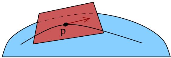
Figure 13. The tangent space at a point $p.$

With a given chart, this curve becomes $\varphi \circ \sigma :\mathbf{R}\mapsto {\mathbf{R}}^n$ , parameterised by $x^{\mu }(t)$ Before we learned any differential geometry, we would say that the tangent vector to the curve at $t=0$ is

$$X^{\mu }={\frac{d{x}^{\mu }(t)}{dt}|}_{t=0}$$

But we can take these to be the components of the tangent vector $X_p,$ , which we define as

$$X_p={\frac{d{x}^{\mu }(t)}{dt}|}_{t=0}{\frac{\partial }{\partial x^{\mu }}|}_p$$

Our tangent vector now acts on functions $f\in C^{\infty }(M)$ . It is telling us how fast any function f changes as we move along the curve.

Any tangent vector $X_p$ can be written in this form. This gives meaning to the term “tangent space” for $T_p(M)$ . It is, literally, the space of all possible tangents to curves passing through the point $p.$ . For example, a two dimensional manifold, embedded in ${\mathbf{R}}^3$ is shown in Figure 13. At each point p, we can identify a vector space which is the tangent plane: this is $T_p(M)$

As an aside, note that the mathematical definition of a tangent space makes no reference to embedding the manifold in some higher dimensional space. The tangent space is an object intrinsic to the manifold itself. (This is in contrast to the picture where it was unfortunately necessary to think about the manifold as embedded in ${\mathbf{R}}^3.$ )

The tangent spaces $T_p(M)$ and $T_q(M)$ at different points $p\ne q$ are different. There’s no sense in which we can add vectors from one to vectors from the other. In fact, at this stage there’s no way to even compare vectors in $T_p(M)$ to vectors in $T_q(M)$ . They are simply different spaces. As we proceed, we will make some effort to figure ways to get around this.

2.2.2 Vector Fields

So far we have only defined tangent vectors at a point p. It is useful to consider an object in which there is a choice of tangent vector for every point $p\in M$ . In physics, we call objects that vary over space fields.

A vector field X is defined to be a smooth assignment of a tangent vector $X_p$ to each point $p\in M$ . This means that if you feed a function to a vector field, then it spits back another function, which is the differentiation of the first. In symbols, a vector field is therefore a map $X:C^{\infty }(M)\to C^{\infty }(M)$ . The function $X(f)$ is defined by

$$(X(f))(p)=X_p(f)$$

The space of all vector fields on M is denoted X(M).

Given a coordinate basis, we can expand any vector field as

$$X=X^{\mu }\frac{\partial }{\partial x^{\mu }}\text{\hspace{1em}(2.7)}$$

where the $X^{\mu }$ are now smooth functions on M.

Strictly speaking, the expression (2.7) only defines a vector field on the open set $\mathcal{O}\subset M$ covered by the chart, rather than the whole manifold. We may have to patch this together with other charts to cover all of M.

The Commutator

Given two vector fields $X,Y\in \mathfrak{X}(M)$ , we can’t multiply them together to get a new vector field. Roughly speaking, this is because the product XY is a second order differential operator rather than a first order operator. This reveals itself in a failure of Leibnizarity for the object XY ,

$$XY(fg)=X(fY(g)+Y(f)g)=X(f)Y(g)+fXY(g)+gXY(f)+X(g)Y(f)$$

This is not the same as $fXY(g)+gXY(f)$ that Leibniz requires.

However, we can build a new vector field by taking the commutator $[X,Y]$ , which acts on functions $f$ as

$$[X,Y](f)=X(Y(f))-Y(X(f))$$

This is also known as the Lie bracket. Evaluated in a coordinate basis, the commutator is given by

$$\begin{array}{c}[X,Y](f)=X^{\mu }\frac{\partial }{\partial x^{\mu }}\left(Y^{\nu }\frac{\partial f}{\partial x^{\nu }}\right)-Y^{\mu }\frac{\partial }{\partial x^{\mu }}\left(X^{\nu }\frac{\partial f}{\partial x^{\nu }}\right)\\ =\left(X^{\mu }\frac{\partial Y^{\nu }}{\partial x^{\mu }}-Y^{\mu }\frac{\partial X^{\nu }}{\partial x^{\mu }}\right)\frac{\partial f}{\partial x^{\nu }}\end{array}$$

This holds for all $f\in C^{\infty }(M)$ , so we’re at liberty to write

$$[X,Y]=\left(X^{\mu }\frac{\partial Y^{\nu }}{\partial x^{\mu }}-Y^{\mu }\frac{\partial X^{\nu }}{\partial x^{\mu }}\right)\frac{\partial }{\partial x^{\nu }}\text{\hspace{1em}(2.8)}$$

It is not difficult to check that the commutator obeys the Jacobi identity

$$[X,[Y,Z]]+[Y,[Z,X]]+[Z,[X,Y]]=0$$

This ensures that the set of all vector fields on a manifold M has the mathematical structure of a Lie algebra.

2.2.3 Integral Curves

There is a slightly different way of thinking about vector fields on a manifold. A flow on M is a one-parameter family of diffeomorphisms ${\sigma }_t:M\to M$ labelled by $t\in \mathbf{R}$ These maps have the properties that ${\sigma }_{t=0}$ is the identity map, and ${\sigma }_s\circ {\sigma }_t={\sigma }_{s+t}$ . These two requirements ensure that ${\sigma }_{-t}={\sigma }_t^{-1}$ . Such a flow gives rise to streamlines on the manifold. We will further require that these streamlines are smooth.

We can then define a vector field by taking the tangent to the streamlines at each point. In a given coordinate system, the components of the vector field are

$$X^{\mu }(x^{\mu }(t))=\frac{d{x}^{\mu }(t)}{dt}\text{\hspace{1em}(2.9)}$$

where I’ve abused notation a little and written $x^{\mu }(t)$ rather than the more accurate but cumbersome $x^{\mu }({\sigma }_t)$ . This will become a habit, with the coordinates $x^{\mu }$ often used to refer to the point $p\in M$

A flow gives rise to a vector field. Alternatively, given a vector field $X^{\mu }(x)$ , we can integrate the differential equation (2.9), subject to an initial condition $x^{\mu }(0)=x_{\mathrm{initial}}^{\mu }$ to generate streamlines which start at $x_{\mathrm{initial}}^{\mu }$ . These streamlines are called integral curves, generated by X.

In what follows, we will only need the infinitesimal flow generated by X. This is simply

$$x^{\mu }(t)=x^{\mu }(0)+t{X}^{\mu }(x)+\mathcal{O}(t^2)\text{\hspace{1em}(2.10)}$$

Indeed, differentiating this obeys (2.9) to leading order in t.

(An aside: Given a vector field X, it may not be possible to integrate (2.9) to generate a flow defined for all $t\in \mathbf{R}$ . For example, consider $M=\mathbf{R}$ with the vector field $X=x^2$ . The equation $dx/dt=x^2$ , subject to the initial condition $x(0)=a$ , has the unique solution $x(t)=a/(1-at)$ which diverges at $t=1/a$ . Vector fields which generate a flow for all $t\in \mathbf{R}$ are called complete. It turns out that all vector fields on a manifold M are complete if M is compact. Roughly speaking, “compact” means that M doesn’t “stretch to infinity”. More precisely, a topological space M is compact if, for any family of open sets covering M there always exists a finite sub-family which also cover M. So R is not compact because the family of sets $\{(-n,n),n\in {\mathbf{Z}}^{+}\}$ covers R but has no finite sub-family. Similarly, ${\mathbf{R}}^n$ is non-compact. However, ${\mathbf{S}}^n$ and ${\mathbf{T}}^n$ are compact manifolds.)

We can look at some examples.

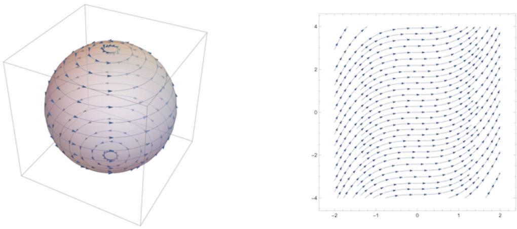
• Consider the sphere ${\mathbf{S}}^2$ in polar coordinates with the vector field $X={\partial }_{\varphi }$ . The integral curves solve the equation (2.9), which are

$$\frac{d\varphi }{dt}=1\mathrm{and}\frac{d\theta }{dt}=0$$

This has the solution $\theta :=:{\theta }_0$ and $\varphi ={\varphi }_0+t$ . The associated one-parameter diffeomorphism is ${\sigma }_t:(\theta ,\varphi )\to (\theta ,\varphi +t)$ , and the flow lines are simply lines of constant latitude on the sphere and are shown in the left-hand figure.

• Alternatively, consider the vector field on ${\mathbf{R}}^2$ with Cartesian components $X^{\mu }=$ $(1,x^2)$ . The equation for the integral curves is now

$$\frac{dx}{dt}=1\mathrm{and}\frac{dy}{dt}=x^2$$

which has the solution $x(t)=x_0+t$ and $\begin{array}{r}y(t)=y_0+\frac{1}{3}(x_0+t{)}^3\end{array}$ . The associated flow lines are shown in the right-hand figure.

2.2.4 The Lie Derivative

So far we have learned how to differentiate a function. This requires us to introduce a vector field X, and the new function $X(f)$ can be viewed as the derivative of $f$ in the direction of X.

Next we ask: is it possible to differentiate a vector field? Specifically, suppose that we have a second vector field Y. How can we differentiate this in the direction of X to get a new vector field? As we’ve seen, we can’t just write down $XY$ because this doesn’t define a new vector field.

To proceed, we should think more carefully about what differentiation means. For a function $f(x)$ on R, we compare the values of the function at nearby points, and see what happens as those points approach each other

$$\frac{df}{dx}=\underset{t\to 0}{\lim }\frac{f(x+t)-f(x)}{t}$$

Similarly, to differentiate a vector field, we need to subtract the tangent vector $Y_p\in$ $T_p(M)$ from the tangent vector at some nearby point $Y_q\in T_q(M)$ , and then see what happens in the limit q → p $q\to p$ . But that’s problematic because, as we stressed above, the vector spaces $T_p(M)$ and $T_q(M)$ are different, and it makes no sense to subtract vectors in one from vectors in the other. To make progress, we’re going to have to find a way to do this. Fortunately, there is a way.

Push-Forward and Pull-Back

Suppose that we have a map $\phi :M\to N$ between two manifolds M and N which we will take to be a diffeomorphism. This allows us to import various structures on one manifold to the other.

For example, if we have a function on $f:N\to \mathbf{R}$ , then we can construct a new function that we denote $({\phi }^{\ast }f):M\to \mathbf{R}$

$$({\phi }^{\ast }f)(p)=f(\phi (p))$$

Using the map in this way, to drag objects originally defined on N onto M is called the pull-back. If we introduce coordinates $x^{\mu }$ on M and $y^{\alpha }$ on $N.$ , then the map $\phi (x)=$ $y^{\alpha }(x)$ , and we can write

$$({\phi }^{\ast }f)(x)=f(y(x))$$

Some objects more naturally go the other way. For example, given a vector field Y on M, we can define a new vector field $({\phi }_{\ast }Y)$ on N. If we are given a function $f:N\to \mathbf{R}$ then the vector field $({\phi }_{\ast }Y)$ on N acts as

$$({\phi }_{\ast }Y)(f)=Y({\phi }^{\ast }f)$$

where I’ve been a little sloppy in the notation here since the left-hand side is a function on N and the right-hand side a function on M. The equality above holds when evaluated at the appropriate points: $[({\phi }_{\ast }Y)(f)](\phi (p))=[Y({\phi }^{\ast }f)](p)$ . Using the map to push objects on M onto N is called the push-forward.

If $Y=Y^{\mu }\partial /\partial x^{\mu }$ is the vector field on M, we can write the induced vector field on $N$ as

$$({\phi }_{\ast }Y)(f)=Y^{\mu }\frac{\partial f(y(x))}{\partial x^{\mu }}=Y^{\mu }\frac{\partial y^{\alpha }}{\partial x^{\mu }}\frac{\partial f(y)}{\partial y^{\alpha }}$$

Written in components, $({\phi }_{\ast }Y)=({\phi }_{\ast }Y{)}^{\alpha }\partial /\partial y^{\alpha }$ , we then have

$$({\phi }_{\ast }Y{)}^{\alpha }=Y^{\mu }\frac{\partial y^{\alpha }}{\partial x^{\mu }}\text{\hspace{1em}(2.11)}$$

Given the way that the indices are contracted, this is more or less the only thing we could write down.

We’ll see other examples of these induced maps later in the lectures. The pushforward is always denoted as ${\phi }_{\ast }$ and goes in the same way as the original map. The pull-back is always denoted as ${\phi }^{\ast }$ and goes in the opposite direction to the original map. Importantly, if our map $\phi :\mathcal{M}\to N$ is a diffeomorphism, then we also have ${\phi }^{-1}:N\to M$ , so we can transport any object from M to N and back again with impunity.

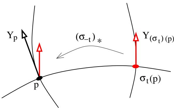
Figure 15. To construct the Lie derivative, we use the push-forward $({\sigma }_{-t}).$ to map the vector $Y_{{\sigma }_t(p)}$ back to p. The resulting vector, shown in red, is $(({\sigma }_{-t}{)}_{\star }Y{)}_p$

Constructing the Lie Derivative

Now we can use these ideas to help build a derivative. Suppose that we are given a vector field X on M. This generates a flow ${\sigma }_t:M\to M$ , which is a map between manifolds, now with $N=M$ . This means that we can use (2.11) to generate a pushforward map from $T_p(M)$ to $T_{{\sigma }_t(p)}(M)$ . But this is exactly what we need if we want to compare tangent vectors at neighbouring points. The resulting differential operator is called the Lie derivative and is denoted ${\mathcal{L}}_X$

It will turn out that we can use these ideas to differentiate many different kinds of objects. As a warm-up, let’s first see how an analogous construction allows us to differentiate functions. Now the function

$${\mathcal{L}}_{X}f=\underset{t\to 0}{\lim }\frac{f({\sigma }_t(x))-f(x)}{t}={\frac{df({\sigma }_t(x))}{dt}|}_{t=0}={\frac{\partial f}{\partial x^{\mu }}\frac{d{x}^{\mu }}{dt}|}_{t=0}$$

But, using (2.9), we know that $d{x}^{\mu }/dt=X^{\mu }$ . We then have

$${\mathcal{L}}_{X}f=X^{\mu }(x)\frac{\partial f}{\partial x^{\mu }}=X(f)\text{\hspace{1em}(2.12)}$$

In other words, acting on functions with the Lie derivative ${\mathcal{L}}_X$ coincides with action of the vector field X.

Now let’s look at the action of ${\mathcal{L}}_X$ on a vector field Y. This is defined by

$${\mathcal{L}}_{X}Y=\underset{t\to 0}{\lim }\frac{(({\sigma }_{-t}{)}_{\ast }Y{)}_p-Y_p}{t}$$

Note the minus sign in ${\sigma }_{-t}$ . This reflects that fact that vector fields are pushed, rather than pulled. The map ${\sigma }_t$ takes us from the point p to the point ${\sigma }_t(p)$ . But to push a tangent vector $Y_{{\sigma }_t(p)}\in \mathrm{\Delta }{T}_{{\sigma }_t(p)}(\mathcal{M})$ to a tangent vector in $T_p(M)$ , where it can be compared to $Y_p$ , we need to push with the inverse map $({\sigma }_{-t}{)}_{\ast }$ . This is shown Figure 15.

Let’s first calculate the action of ${\mathcal{L}}_X$ on a coordinate basis ${\partial }_{\mu }=\partial /\partial x^{\mu }$ . We have

$${\mathcal{L}}_X{\partial }_{\mu }=\underset{t\to 0}{\lim }\frac{({\sigma }_{-t}{)}_{\ast }{\partial }_{\mu }-{\partial }_{\mu }}{t}\text{\hspace{1em}(2.13)}$$

We have an expression for the push-forward of a tangent vector in (2.11), where the coordinates $y^{\alpha }$ on N should now be replaced by the infinitesimal change of coordinates induced by the flow ${\sigma }_{-t}$ which, from (2.10) is $x^{\mu }(t)=x^{\mu }(0)-t{X}^{\mu }+....$ Note the minus sign, which comes from the fact that we have to map back to where we came from as shown in Figure 15. We have, for small $t,$

$$({\sigma }_{-t}{)}_{\ast }{\partial }_{\mu }=\left({\delta }_{\mu }^{\nu }-t\frac{\partial X^{\nu }}{\partial x^{\mu }}+\dots \right){\partial }_{\nu }$$

Acting on a coordinate basis, we then have

$${\mathcal{L}}_X{\partial }_{\mu }=-\frac{\partial X^{\nu }}{\partial x^{\mu }}{\partial }_{\nu }\text{\hspace{1em}(2.14)}$$

To determine the action of ${\mathcal{L}}_X$ on a general vector field Y, we use the fact that the Lie derivative obeys the usual properties that we expect of a derivative, including linearity, ${\mathcal{L}}_X(Y_1+Y_2)={\mathcal{L}}_X{Y}_1+{\mathcal{L}}_X{Y}_2$ and Leibnizarity ${\mathcal{L}}_X(fY)=f{\mathcal{L}}_{X}Y+({\mathcal{L}}_{X}f)Y$ for any function $f$ , both of which follow from the definition. The action on a general vector field $Y=Y^{\mu }(x)\partial /\partial x^{\mu }$ can then be written as

$${\mathcal{L}}_X(Y^{\mu }{\partial }_{\mu })=({\mathcal{L}}_X{Y}^{\mu }){\partial }_{\mu }+Y^{\mu }({\mathcal{L}}_X{\partial }_{\mu })$$

where we’ve simply viewed the components $Y^{\mu }(x)$ as n functions. We can use (2.12) to determine ${\mathcal{L}}_X{Y}^{\mu }$ and we’ve computed ${\mathcal{L}}_X{\partial }_{\mu }$ in (2.14). We then have

$${\mathcal{L}}_X(Y^{\mu }{\partial }_{\mu })=X^{\nu }\frac{\partial Y^{\mu }}{\partial x^{\nu }}{\partial }_{\mu }-Y^{\mu }\frac{\partial X^{\nu }}{\partial x^{\mu }}{\partial }_{\nu }$$

But this is precisely the structure of the commutator. We learn that the Lie derivative acting on vector fields is given by

$${\mathcal{L}}_{X}Y=[X,Y]$$

A corollary of this is

$${\mathcal{L}}_X{\mathcal{L}}_{Y}Z-{\mathcal{L}}_Y{\mathcal{L}}_{X}Z={\mathcal{L}}_{[X,Y]}Z\text{\hspace{1em}(2.15)}$$

which follows from the Jacobi identity for commutators.

The Lie derivative is just one of several derivatives that we will meet in this course. As we introduce new objects, we will learn how to act with ${\mathcal{L}}_X$ on them. But we will also see that we can endow different meanings to the idea of differentiation. In fact, the Lie derivative will take something of a back seat until Section 4.3 when we will see that it is what we need to understand symmetries.

来源与版本

正文：英文 · OCR 机器稿 · 待校对

核对状态：OCR 机器稿 · 待校对

原书 PDF

来源版本：michaelmas-2019-source-20260923

来源 PDF SHA-256：3ba65dc61f22a69c7d5fdf3e8e1f641efbfa6cf49a44b3dcb0fd5367ba9fcf1c

OCR 来源 SHA-256：f58e775c8ca9f14ce79c624d8e60dcf8f6b8feacb94e5342e9bfd0dc174328a5

OCR 产物 SHA-256：f25c11d2bfb02b6fe569572a5efb5b852d47ba0302f54ca7c6733a45427c3f3b