5.2 The calculus on manifolds

The significance of differentiable manifolds resides in the fact that we may use the usual calculus developed in ${\mathbb{R}}^n$ . Smoothness of the coordinate transformations

ensures that the calculus is independent of the coordinates chosen.

5.2.1 Differentiable maps

Let $f:M\to N$ be a map from an $m$ -dimensional manifold $M$ to an $n$ -dimensional manifold $N$ . A point $p\in M$ is mapped to a point $f(p)\in N$ , namely $f:p\mapsto f(p)$ , see figure 5.6. Take a chart $(U,\phi )$ on $M$ and $(V,\psi )$ on $N$ , where $p\in U$ and $f(p)\in V$ . Then $f$ has the following coordinate presentation:

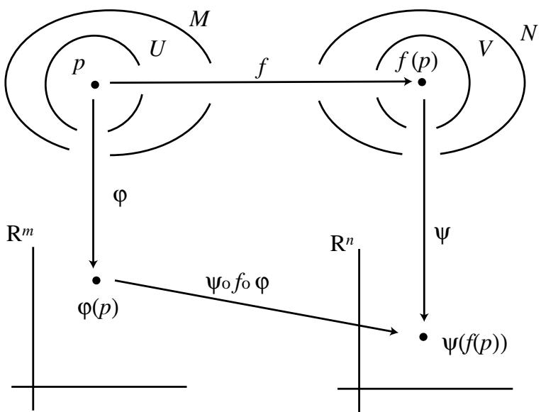
Figure 5.6. A map $f:M\to N$ has a coordinate presentation $\psi \circ f\circ {\phi }^{-1}:{\mathbb{R}}^m\to {\mathbb{R}}^n$ .

$$\psi \circ f\circ {\phi }^{-1}:{\mathbb{R}}^m\to {\mathbb{R}}^n.\text{\hspace{1em}(5.16)}$$

If we write $\phi (p)=\{x^{\mu }\}$ and $\psi (f(p))=\{y^{\alpha }\}$ , $\psi \circ f\circ {\phi }^{-1}$ is just the usual vector-valued function $y=\psi \circ f\circ {\phi }^{-1}(x)$ of $m$ variables. We sometimes use (in fact, abuse!) the notation $y=f(x)$ or $y^{\alpha }=f^{\alpha }(x^{\mu })$ , when we know which coordinate systems on $M$ and $N$ are in use. If $y=\psi \circ f\circ {\phi }^{-1}(x)$ , or simply $y^{\alpha }=f^{\alpha }(x^{\mu })$ , is $C^{\infty }$ with respect to each $x^{\mu }$ , $f$ is said to be differentiable at $p$ or at $x=\phi (p)$ . Differentiable maps are also said to be smooth. Note that we require infinite ( $C^{\infty }$ ) differentiability, in harmony with the smoothness of the transition functions ${\psi }_{ij}$ .

The differentiability of $f$ is independent of the coordinate system. Consider two overlapping charts $(U_1,{\phi }_1)$ and $(U_2,{\phi }_2)$ . Take a point $p\in U_1\cap U_2$ , whose coordinates by ${\phi }_1$ are $\{x_1^{\mu }\}$ , while those by ${\phi }_2$ are $\{x_2^{\nu }\}$ . When expressed in terms of $\{x_1^{\mu }\}$ , $f$ takes the form $\psi \circ f\circ {\phi }_1^{-1}$ , while in $\{x_2^{\nu }\}$ , $\psi \circ f\circ {\phi }_2^{-1}=$

$\psi \circ f\circ {\phi }_1^{-1}({\phi }_1\circ {\phi }_2^{-1})$ . By definition, ${\psi }_{12}={\phi }_1\circ {\phi }_2^{-1}$ is $C^{\infty }$ . In the simpler expressions, they correspond to $y=f(x_1)$ and $y=f(x_1(x_2))$ . It is clear that if $f(x_1)$ is $C^{\infty }$ with respect to $x_1^{\mu }$ and $x_1(x_2)$ is $C^{\infty }$ with respect to $x_2^{\nu }$ , then $y=f(x_1(x_2))$ is also $C^{\infty }$ with respect to $x_2^{\nu }$ .

Exercise 5.2

Show that the differentiability of $f$ is also independent of the chart in $N$ .

Definition 5.2

Let $f:M\to N$ be a homeomorphism and $\psi$ and $\phi$ be coordinate functions as previously defined. If $\psi \circ f\circ {\phi }^{-1}$ is invertible (that is, there exists a map $\phi \circ f^{-1}\circ {\psi }^{-1}$ ) and both $y=\psi \circ f\circ {\phi }^{-1}(x)$ and $x=\phi \circ f^{-1}\circ {\psi }^{-1}(y)$ are $C^{\infty }$ , $f$ is called a diffeomorphism and $M$ is said to be diffeomorphic to $N$ and vice versa, denoted by $M\equiv N$ .

Clearly $\dim M=\dim N$ if $M\equiv N$ . In chapter 2, we noted that homeomorphisms classify spaces according to whether it is possible to deform one space into another continuously. Diffeomorphisms classify spaces into equivalence classes according to whether it is possible to deform one space to another smoothly. Two diffeomorphic spaces are regarded as the same manifold. Clearly a diffeomorphism is a homeomorphism. What about the converse? Is a homeomorphism a diffeomorphism? In the previous section, we defined the differentiable structure as an equivalence class of atlases. Is it possible for a topological space to carry many differentiable structures? It is rather difficult to give examples of ‘diffeomorphically inequivalent homeomorphisms’ since it is known that this is possible only in higher-dimensional spaces (dim $M\ge 4$ ). It was believed before 1956 that a topological space admits only one differentiable structure. However, Milnor (1956) pointed out that $S^7$ admits 28 differentiable structures. A recent striking discovery in mathematics is that ${\mathbb{R}}^4$ admits an infinite number of differentiable structures. Interested readers should consult Donaldson (1983) and Freed and Uhlenbeck (1984). Here we assume that a manifold admits a unique differentiable structure, for simplicity.

The set of diffeomorphisms $f:M\to M$ is a group denoted by $\mathrm{Diff}(M)$ . Take a point $p$ in a chart $(U,\phi )$ such that $\phi (p)=x^{\mu }(p)$ . Under $f\in \mathrm{Diff}(M)$ , $p$ is mapped to $f(p)$ whose coordinates are $\phi (f(p))=y^{\mu }(f(p))$ (we have assumed $f(p)\in U$ ). Clearly $y$ is a differentiable function of $x$ ; this is an active point of view to the coordinate transformation. However, if $(U,\phi )$ and $(V,\psi )$ are overlapping charts, we have two coordinate values $x^{\mu }=\phi (p)$ and $y^{\mu }=\psi (p)$ for a point $p\in U\cap V$ . The map $x\mapsto y$ is differentiable by the assumed smoothness of the manifold; this reparametrization is a passive point of view to the coordinate transformation. We also denote the group of reparametrizations by $\mathrm{Diff}(M)$ .

Now we look at special classes of mappings, namely curves and functions. An open curve in an $m$ -dimensional manifold $M$ is a map $c:(a,b)\to M$ where $(a,b)$ is an open interval such that $a<0<b$ . We assume that the curve does not intersect with itself (figure 5.7). The number $a(b)$ may be $-\infty (+\infty )$ and we have included 0 in the interval for later convenience. If a curve is closed, it is

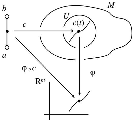
Figure 5.7. A curve $c$ in $M$ and its coordinate presentation $\phi \circ c$ .

regarded as a map $c:S^1\to M$ . In both cases, $c$ is locally a map from an open interval to $M$ . On a chart $(U,\phi )$ , a curve $c(t)$ has the coordinate presentation $x=\phi \circ c:\mathbb{R}\to {\mathbb{R}}^m$ .

A function $f$ on $M$ is a smooth map from $M$ to $\mathbb{R}$ , see figure 5.8. On a chart $(U,\phi )$ , the coordinate presentation of $f$ is given by $f\circ {\phi }^{-1}:{\mathbb{R}}^m\to \mathbb{R}$ which is a real-valued function of $m$ variables. We denote the set of smooth functions on $M$ by $\mathcal{F}(M)$ .

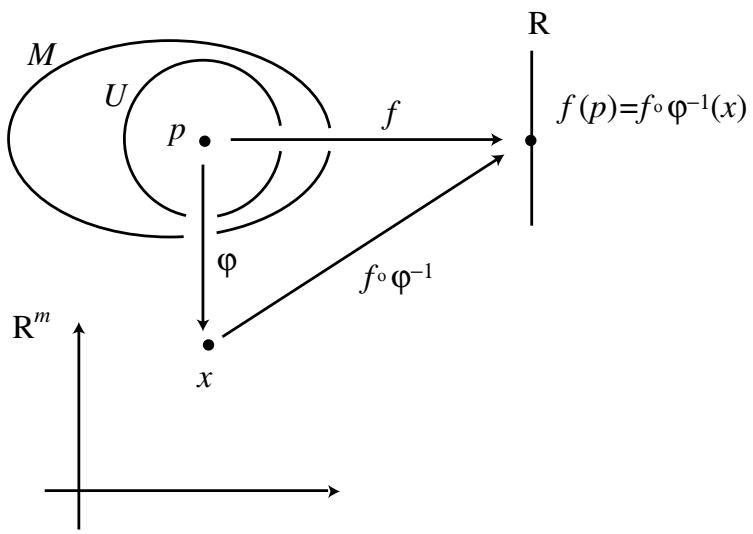
Figure 5.8. A function $f:M\to \mathbb{R}$ and its coordinate presentation $f\circ {\phi }^{-1}$ .

5.2.2 Vectors

Now that we have defined maps on a manifold, we are ready to define other geometrical objects: vectors, dual vectors and tensors. In general, an elementary picture of a vector as an arrow connecting a point and the origin does not work in a manifold. [Where is the origin? What is a straight arrow? How do we define a straight arrow that connects London and Los Angeles on the surface of the Earth?] On a manifold, a vector is defined to be a tangent vector to a curve in $M$ .

To begin with, let us look at a tangent line to a curve in the $xy$ -plane. If the curve is differentiable, we may approximate the curve in the vicinity of $x_0$ by

$$y-y\left(x_0\right)=a\left(x-x_0\right)\text{\hspace{1em}(5.17)}$$

where $a=\mathrm{dy}/\mathrm{dx}{|}_{x=x_0}$ . The tangent vectors on a manifold $M$ generalize this tangent line. To define a tangent vector we need a curve $c:(a,b)\to M$ and a function $f:M\to \mathbb{R}$ , where $(a,b)$ is an open interval containing $t=0$ , see figure 5.9. We define the tangent vector at $c(0)$ as a directional derivative of a function $f(c(t))$ along the curve $c(t)$ at $t=0$ . The rate of change of $f(c(t))$ at

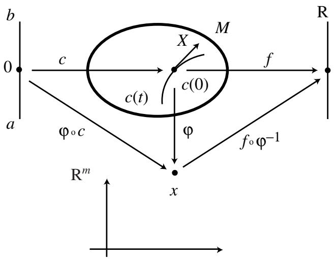
Figure 5.9. A curve $c$ and a function $f$ define a tangent vector along the curve in terms of the directional derivative.

$t=0$ along the curve is

$${\frac{\mathrm{d}f(c(t))}{\mathrm{d}t}|}_{t=0}.\text{\hspace{1em}(5.18)}$$

In terms of the local coordinate, this becomes

$${\frac{\partial f}{\partial x^{\mu }}\frac{\mathrm{d}{x}^{\mu }(c(t))}{\mathrm{d}t}|}_{t=0}.\text{\hspace{1em}(5.19)}$$

[Note the abuse of the notation! The derivative $\partial f/\partial x^{\mu }$ really means $\partial (f\circ {\phi }^{-1}(x))/\partial x^{\mu }.$ ] In other words, $\mathrm{d}f(c(t))/\mathrm{d}t$ at $t=0$ is obtained by applying the differential operator $X$ to $f$ , where

$$X=X^{\mu }\left(\frac{\partial }{\partial x^{\mu }}\right)\left(X^{\mu }=\frac{\mathrm{d}{x}^{\mu }(c(t))}{\mathrm{d}t}{|}_{t=0}\right)(5.20)$$

that is,

$${\frac{\mathrm{d}f(c(t))}{\mathrm{d}t}|}_{t=0}=X^{\mu }\left(\frac{\partial f}{\partial x^{\mu }}\right)\equiv X[f].\text{\hspace{1em}(5.21)}$$

Here the last equality defines $X[f]$ . It is $X=X^{\mu }\partial /\partial x^{\mu }$ which we now define as the tangent vector to $M$ at $p=c(0)$ along the direction given by the curve $c(t)$ .

Example 5.7

If $X$ is applied to the coordinate functions $\phi (c(t))=x^{\mu }(t)$ , we have

$$X[x^{\mu }]=\left(\frac{\mathrm{d}{x}^{\nu }}{\mathrm{d}t}\right)\left(\frac{\partial x^{\mu }}{\partial x^{\nu }}\right)={\frac{\mathrm{d}{x}^{\mu }(t)}{\mathrm{d}t}|}_{t=0}$$

which is the $\mu$ th component of the velocity vector if $t$ is understood as time.

To be more mathematical, we introduce an equivalence class of curves in $M$ . If two curves $c_1(t)$ and $c_2(t)$ satisfy

(i) $c_1(0)=c_2(0)=p$
(ii) ${\frac{\mathrm{d}{x}^{\mu }(c_1(t))}{\mathrm{d}t}|}_{t=0}={\frac{\mathrm{d}{x}^{\mu }(c_2(t))}{\mathrm{d}t}|}_{t=0}$

$c_1(t)$ and $c_2(t)$ yield the same differential operator $X$ at $p$ , in which case we define $c_1(t)\sim c_2(t)$ . Clearly $\sim$ is an equivalence relation and defines the equivalence classes. We identify the tangent vector $X$ with the equivalence class of curves

$$[c(t)]=\left\{\tilde{c}(t)\mid \tilde{c}(0)=c(0)\text{a n d}\frac{\mathrm{d}{x}^{\mu }(\tilde{c}(t))}{\mathrm{d}t}{|}_{t=0}=\frac{\mathrm{d}{x}^{\mu }(c(t))}{\mathrm{d}t}{|}_{t=0}\right\}\text{\hspace{1em}(5.22)}$$

rather than a curve itself.

All the equivalence classes of curves at $p\in M$ , namely all the tangent vectors at $p$ , form a vector space called the tangent space of $M$ at $p$ , denoted by $T_{p}M$ . To analyse $T_{p}M$ , we may use the theory of vector spaces developed in section 2.2. Evidently, $e_{\mu }=\partial /\partial x^{\mu }$ ( $1\le \mu \le m$ ) are the basis vectors of $T_{p}M$ , see (5.20), and $\dim T_{p}M=\dim M$ . The basis $\{e_{\mu }\}$ is called the coordinate basis. If a vector $V\in T_{p}M$ is written as $V=V^{\mu }{e}_{\mu }$ , the numbers $V^{\mu }$ are called the components of $V$ with respect to $e_{\mu }$ . By construction, it is obvious that a vector $X$ exists without specifying the coordinate, see (5.21). The assignment of

the coordinate is simply for our convenience. This coordinate independence of a vector enables us to find the transformation property of the components of the vector. Let $p\in U_i\cap U_j$ and $x={\phi }_i(p),y={\phi }_j(p)$ . We have two expressions for $X\in T_{p}M$ ,

$$X=X^{\mu }\frac{\partial }{\partial x^{\mu }}={\tilde{X}}^{\mu }\frac{\partial }{\partial y^{\mu }}.$$

This shows that $X^{\mu }$ and ${\tilde{X}}^{\mu }$ are related as

$${\tilde{X}}^{\mu }=X^{\nu }\frac{\partial y^{\mu }}{\partial x^{\nu }}.\text{\hspace{1em}(5.23)}$$

Note again that the components of the vector transform in such a way that the vector itself is left invariant.

The basis of $T_{p}M$ need not be $\{e_{\mu }\}$ , and we may think of the linear combinations ${\hat{e}}_i\equiv A_i^{\mu }{e}_{\mu }$ , where $A=(A_i^{\mu })\in \mathrm{GL}(m,\mathbb{R})$ . The basis $\{{\hat{e}}_i\}$ is known as the non-coordinate basis.

5.2.3 One-forms

Since $T_{p}M$ is a vector space, there exists a dual vector space to $T_{p}M$ , whose element is a linear function from $T_{p}M$ to $\mathbb{R}$ , see section 2.2. The dual space is called the cotangent space at $p$ , denoted by $T_p^{\ast }M$ . An element $\omega :T_{p}M\to \mathbb{R}$ of $T_p^{\ast }M$ is called a dual vector, cotangent vector or, in the context of differential forms, a one-form. The simplest example of a one-form is the differential $\mathrm{d}f$ of a function $f\in \mathcal{F}(M)$ . The action of a vector $V$ on $f$ is $V[f]=V^{\mu }\partial f/\partial x^{\mu }\in \mathbb{R}$ . Then the action of $\mathrm{d}f\in T_p^{\ast }M$ on $V\in T_{p}M$ is defined by

$$⟨\mathrm{d}f,V⟩\equiv V[f]=V^{\mu }\frac{\partial f}{\partial x^{\mu }}\in \mathbb{R}.\text{\hspace{1em}(5.24)}$$

Clearly $⟨\mathrm{d}f,V⟩$ is $\mathbb{R}$ -linear in both $V$ and $f$

Noting that $\mathrm{df}$ is expressed in terms of the coordinate $x=\phi (p)$ as $\mathrm{df}=(\partial f/\partial x^{\mu }){\mathrm{dx}}^{\mu }$ , it is natural to regard $\{{\mathrm{dx}}^{\mu }\}$ as a basis of $T_p^{\ast }M$ . Moreover, this is a dual basis, since

$$⟨\mathrm{d}{x}^{\mu },\frac{\partial }{\partial x^{\mu }}⟩=\frac{\partial x^{\nu }}{\partial x^{\mu }}={\delta }_{\mu }^{\nu }.\text{\hspace{1em}(5.25)}$$

An arbitrary one-form $\omega$ is written as

$$\omega ={\omega }_{\mu }\mathrm{d}{x}^{\mu }\text{\hspace{1em}(5.26)}$$

where the ${\omega }_{\mu }$ are the components of $\omega$ . Take a vector $V=V^{\mu }\partial /\partial x^{\mu }$ and a one-form $\omega ={\omega }_{\mu }\mathrm{d}{x}^{\mu }$ . The inner product $⟨,⟩:T_p^{\ast }M\times T_{p}M\to \mathbb{R}$ is defined by

$$⟨\omega ,V⟩={\omega }_{\mu }{V}^v⟨\mathrm{d}{x}^{\mu },\frac{\partial }{\partial x^v}⟩={\omega }_{\mu }{V}^v{\delta }_v^{\mu }={\omega }_{\mu }{V}^{\mu }.\text{\hspace{1em}(5.27)}$$

Note that the inner product is defined between a vector and a dual vector and not between two vectors or two dual vectors.

Since $\omega$ is defined without reference to any coordinate system, for a point $p\in U_i\cap U_j$ , we have

$$\omega ={\omega }_{\mu }d{x}^{\mu }={\tilde{\omega }}_{v}d{y}^v$$

where $x={\phi }_i(p)$ and $y={\phi }_j(p)$ . From ${\mathrm{dy}}^{\nu }=(\partial y^{\nu }/\partial x^{\mu }){\mathrm{dx}}^{\mu }$ we find that

$${\tilde{\omega }}_v={\omega }_{\mu }\frac{\partial x^{\mu }}{\partial y^v}.\text{\hspace{1em}(5.28)}$$

5.2.4 Tensors

A tensor of type $(q,r)$ is a multilinear object which maps $q$ elements of $T_p^{\ast }M$ and $r$ elements of $T_{p}M$ to a real number. ${\mathfrak{T}}_{r,p}^q(M)$ denotes the set of type $(q,r)$ tensors at $p\in M$ . An element of ${\mathfrak{T}}_{r,p}^q(M)$ is written in terms of the bases described earlier as

$$T=T_{v_1\dots v_r}^{{\mu }_1\dots {\mu }_q}\frac{\partial }{\partial x^{{\mu }_1}}\dots \frac{\partial }{\partial x^{{\mu }_q}}d{x}^{v_1}\dots d{x}^{v_r}.\text{\hspace{1em}(5.29)}$$

Clearly this is a linear function from

$${\otimes }^q{T}_p^{\ast }M{\otimes }^r{T}_{p}M$$

to $\mathbb{R}$ . Let $V_i=V_i^{\mu }\partial /\partial x^{\mu }$ $(1\le i\le r)$ and ${\omega }_i={\omega }_{i\mu }\mathrm{d}{x}^{\mu }$ $(1\le i\le q)$ . The action of $T$ on them yields a number

$$T\left({\omega }_1,\dots ,{\omega }_q;V_1,\dots ,V_r\right)=T_{v_1\dots v_r}^{{\mu }_1\dots {\mu }_q}{\omega }_{1{\mu }_1}\dots {\omega }_{q{\mu }_q}{V}_1^{v_1}\dots V_r^{v_r}.$$

In the present notation, the inner product is $⟨\omega ,X⟩=\omega (X)$

5.2.5 Tensor fields

If a vector is assigned smoothly to each point of $M$ , it is called a vector field over $M$ . In other words, $V$ is a vector field if $V[f]\in \mathcal{F}(M)$ for any $f\in \mathcal{F}(M)$ . Clearly each component of a vector field is a smooth function from $M$ to $\mathbb{R}$ . The set of the vector fields on $M$ is denoted as $\mathcal{X}(M)$ . A vector field $X$ at $p\in M$ is denoted by $X{|}_p$ , which is an element of $T_{p}M$ . Similarly, we define a tensor field of type $(q,r)$ by a smooth assignment of an element of ${\mathfrak{T}}_{r,p}^q(M)$ at each point $p\in M$ . The set of the tensor fields of type $(q,r)$ on $M$ is denoted by ${\mathfrak{T}}_r^q(M)$ . For example, ${\mathfrak{T}}_1^0(M)$ is the set of the dual vector fields, which is also denoted by ${\Omega }^1(M)$ in the context of differential forms, see section 5.4. Similarly, ${\mathfrak{T}}_0^0(M)=\mathcal{F}(M)$ is denoted by ${\Omega }^0(M)$ in the same context.

5.2.6 Induced maps

A smooth map $f:M\to N$ naturally induces a map $f_{\ast }$ called the differential map (figure 5.10),

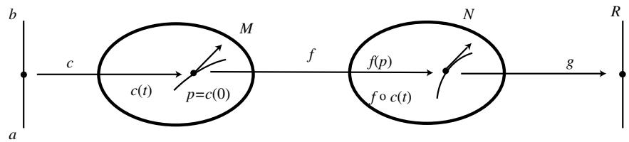
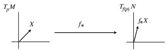
Figure 5.10. A map $f:M\to N$ induces the differential map $f_{\ast }:T_{p}M\to T_{f(p)}N$ .

$$f_{\ast }:T_{p}M\to T_{f(p)}N.\text{\hspace{1em}(5.30)}$$

The explicit form of $f_{\ast }$ is obtained by the definition of a tangent vector as a directional derivative along a curve. If $g\in \mathcal{F}(N)$ , then $g\circ f\in \mathcal{F}(M)$ . A vector $V\in T_{p}M$ acts on $g\circ f$ to give a number $V[g\circ f]$ . Now we define $f_{\ast }V\in T_{f(p)}N$ by

$$\left(f_{\ast }V\right)[g]\equiv V[g\circ f]\text{\hspace{1em}(5.31)}$$

or, in terms of charts $(U,\phi )$ on $M$ and $(V.\psi )$ on $N$ ,

$$\left(f_{\ast }V\right)\left[g\circ {\psi }^{-1}(y)\right]\equiv V\left[g\circ f\circ {\phi }^{-1}(x)\right]\text{\hspace{1em}(5.32)}$$

where $x=\phi (p)$ and $y=\psi (f(p))$ . Let $V=V^{\mu }\partial /\partial x^{\mu }$ and $f_{\ast }V=W^{\alpha }\partial /\partial y^{\alpha }$ . Then (5.32) yields

$$W^{\alpha }\frac{\partial }{\partial y^{\alpha }}[g\circ {\psi }^{-1}(y)]=V^{\mu }\frac{\partial }{\partial x^{\mu }}[g\circ f\circ {\phi }^{-1}(x)].$$

If we take $g=y^{\alpha }$ , we obtain the relation between $W^{\alpha }$ and $V^{\mu }$ ,

$$W^{\alpha }=V^{\mu }\frac{\partial }{\partial x^{\mu }}{y}^{\alpha }(x).\text{\hspace{1em}(5.33)}$$

Note that the matrix $(\partial y^{\alpha }/\partial x^{\mu })$ is nothing but the Jacobian of the map $f:M\to N$ . The differential map $f_{\ast }$ is naturally extended to tensors of type $(q,0)$ , $f_{\ast }:{\mathcal{T}}_{0,p}^q(M)\to {\mathcal{T}}_{0,f(p)}^q(N)$ .

Example 5.8

Let $(x^1,x^2)$ and $(y^1,y^2,y^3)$ be the coordinates in $M$ and $N$ , respectively, and let $V=a\partial /\partial x^1+b\partial /\partial x^2$ be a tangent vector at $(x^1,x^2)$ .

Let $f:M\to N$ be a map whose coordinate presentation is $y=(x^1,x^2,\sqrt{1-(x^1{)}^2-(x^2{)}^2})$ . Then

$$f_{\ast }V=V^{\mu }\frac{\partial y^{\alpha }}{\partial x^{\mu }}\frac{\partial }{\partial y^{\alpha }}=a\frac{\partial }{\partial y^1}+b\frac{\partial }{\partial y^2}-\left(a\frac{y^1}{y^3}+b\frac{y^2}{y^3}\right)\frac{\partial }{\partial y^3}.$$

Exercise 5.3

Let $f:M\to N$ and $g:N\to P$ . Show that the differential map of the composite map $g\circ f:M\to P$ is

$$(g\circ f{)}_{\ast }=g_{\ast }\circ f_{\ast }.\text{\hspace{1em}(5.34)}$$

A map $f:M\to N$ also induces a map

$$f^{\ast }:T_{f(p)}^{\ast }N\to T_p^{\ast }M.\text{\hspace{1em}(5.35)}$$

Note that $f_{\ast }$ goes in the same direction as $f$ , while $f^{\ast }$ goes backward, hence the name pullback, see section 2.2. If we take $V\in T_{p}M$ and $\omega \in T_{f(p)}^{\ast }N$ , the pullback of $\omega$ by $f^{\ast }$ is defined by

$$⟨f^{\ast }\omega ,V⟩=⟨\omega ,f_{\ast }V⟩.\text{\hspace{1em}(5.36)}$$

The pullback $f^{\ast }$ naturally extends to tensors of type $(0,r)$ , $f^{\ast }:{\mathcal{T}}_{r,f(p)}^0(N)\to {\mathcal{T}}_{r,p}^0(M)$ . The component expression of $f^{\ast }$ is given by the Jacobian matrix $(\partial y^{\alpha }/\partial x^{\mu })$ , see exercise 5.4.

Exercise 5.4

Let $f:M\to N$ be a smooth map. Show that for $\omega ={\omega }_{\alpha }\mathrm{d}{y}^{\alpha }\in T_{f(p)}^{\ast }N$ , the induced one-form $f^{\ast }\omega ={\xi }_{\mu }\mathrm{d}{x}^{\mu }\in T_p^{\ast }M$ has components

$${\xi }_{\mu }={\omega }_{\alpha }\frac{\partial y^{\alpha }}{\partial x^{\mu }}.\text{\hspace{1em}(5.37)}$$

Exercise 5.5

Let $f$ and $g$ be as in exercise 5.3. Show that the pullback of the composite map $g\circ f$ is

$$(g\circ f{)}^{\ast }=f^{\ast }\circ g^{\ast }.\text{\hspace{1em}(5.38)}$$

There is no natural extension of the induced map for a tensor of mixed type. The extension is only possible if $f:M\to N$ is a diffeomorphism, where the Jacobian of $f^{-1}$ is also defined.

Exercise 5.6

Let

$$T_v^{\mu }\frac{\partial }{\partial x^{\mu }}\otimes \mathrm{d}{x}^v$$

be a tensor field of type $(1,1)$ on $M$ and let $f:M\to N$ be a diffeomorphism. Show that the induced tensor on $N$ is

$$f_{\ast }\left(T_v^{\mu }\frac{\partial }{\partial x^{\mu }}\otimes \mathrm{d}{x}^v\right)=T_v^{\mu }\left(\frac{\partial y^{\alpha }}{\partial x^{\mu }}\right)\left(\frac{\partial x^v}{\partial y^{\beta }}\right)\frac{\partial }{\partial y^{\alpha }}\otimes \mathrm{d}{y}^{\beta }$$

where $x^{\mu }$ and $y^{\alpha }$ are local coordinates in $M$ and $N$ , respectively.

5.2.7 Submanifolds

Before we close this section, we define a submanifold of a manifold. The meaning of embedding is also clarified here.

Definition 5.3 · Immersion, submanifold, embedding

Let $f:M\to N$ be a smooth map and let $\dim M\le \dim N$ .

(a) The map $f$ is called an immersion of $M$ into $N$ if $f_{\ast }:T_{p}M\to T_{f(p)}N$ is an injection (one to one), that is $\mathrm{rank}{f}_{\ast }=\dim M$ .
(b) The map $f$ is called an embedding if $f$ is an injection and an immersion. The image $f(M)$ is called a submanifold of $N$ . [In practice, $f(M)$ thus defined is diffeomorphic to $M$ .]

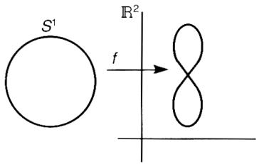
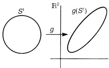
If $f$ is an immersion, $f^{\ast }$ maps $T_{p}M$ isomorphically to an $m$ -dimensional vector subspace of $T_{f(p)}N$ since $\mathrm{rank}{f}_{\ast }=\dim M$ . From theorem 2.1, we also find $\ker f_{\ast }=\{0\}$ . If $f$ is an embedding, $M$ is diffeomorphic to $f(M)$ . Examples will clarify these rather technical points. Consider a map $f:S^1\to {\mathbb{R}}^2$ in figure 5.11(a). It is an immersion since a one-dimensional tangent space of $S^1$ is mapped by $f_{\ast }$ to a subspace of $T_{f(p)}{\mathbb{R}}^2$ . The image $f(S^1)$ is not a submanifold of ${\mathbb{R}}^2$ since $f$ is not an injection. The map $g:S^1\to {\mathbb{R}}^2$ in figure 5.11(b) is an embedding and $g(S^1)$ is a submanifold of ${\mathbb{R}}^2$ . Clearly, an embedding is an immersion although the converse is not necessarily true. In the previous section, we occasionally mentioned the embedding of $S^n$ into ${\mathbb{R}}^{n+1}$ . Now this meaning is clear; if $S^n$ is embedded by $f:S^n\to {\mathbb{R}}^{n+1}$ then $S^n$ is diffeomorphic to $f(S^n)$ .

(a)

(b)

Figure 5.11. (a) An immersion $f$ which is not an embedding. (b) An embedding $g$ and the submanifold $g(S^1)$ .

来源与版本

正文：英文 · OCR 机器稿 · 待校对

核对状态：OCR 机器稿 · 待校对

原书 PDF

来源版本：second-edition-local

来源 PDF SHA-256：fcd24c3371d092a8c699ccf5cf0765462924b6c48412804231076e8084b1940d

OCR 来源 SHA-256：0b6324f01172a3548cd34382e82fd8bfae574602b6b2cfaa357ba96bc2c35478

OCR 产物 SHA-256：97da6b8fd6116b1d4681100026d110fc8b72bbaba5e12c2aa2db99048abba293