7.3 Curvature and torsion

7.3.1 Definitions

Since $\Gamma$ is not a tensor, it cannot have an intrinsic geometrical meaning as a measure of how much a manifold is curved. For example, the connection coefficients in example 7.1 vanish if the Cartesian coordinate is employed while they do not in polar coordinates. As intrinsic objects, we define the torsion tensor

$T:\mathcal{X}(M)\otimes \mathcal{X}(M)\to \mathcal{X}(M)$ and the Riemann curvature tensor (or Riemann tensor) $R:\mathcal{X}(M)\otimes \mathcal{X}(M)\otimes \mathcal{X}(M)\to \mathcal{X}(M)$ by

$$T(X,Y)\equiv {\nabla }_{X}Y-{\nabla }_{Y}X-[X,Y]\text{\hspace{1em}(7.36)}$$

$$R(X,Y,Z)\equiv {\nabla }_X{\nabla }_{Y}Z-{\nabla }_Y{\nabla }_{X}Z-{\nabla }_{[X,Y]}Z.\text{\hspace{1em}(7.37)}$$

It is common to write $R(X,Y)Z$ instead of $R(X,Y,Z)$ , so that $R$ looks like an operator acting on $Z$ . Clearly, they satisfy

$$T(X,Y)=-T(Y,X),R(X,Y)Z=-R(Y,X)Z.\text{\hspace{1em}(7.38)}$$

At first sight, $T$ and $R$ seem to be differential operators and it is not obvious that they are multilinear objects. We prove the tensorial property of $R$ ,

$$\begin{array}{rl}& \\ & R(fX,gY)hZ=f{\nabla }_X\left\{g{\nabla }_Y(hZ)\right\}-g{\nabla }_Y\left\{f{\nabla }_X(hZ)\right\}-fX[g]{\nabla }_Y(hZ)\\ & \\ & +gY[f]{\nabla }_X(hZ)-fg{\nabla }_{[X,Y]}(hZ)\\ & =fg{\nabla }_X\{Y[h]Z+h{\nabla }_{Y}Z\}-gf{\nabla }_Y\{X[h]Z+h{\nabla }_{X}Z\}\\ & -fg[X,Y][h]Z-fgh{\nabla }_{[X,Y]}Z\\ & =fgh\left\{{\nabla }_X{\nabla }_{Y}Z-{\nabla }_Y{\nabla }_{X}Z-{\nabla }_{[X,Y]}Z\right\}\\ & =fghR(X,Y)Z.\end{array}$$

Now it is easy to see that $R$ satisfies

$$R(X,Y)Z=X^{\lambda }{Y}^{\mu }{Z}^{\nu }R\left(e_{\lambda },e_{\mu }\right)e_{\nu }\text{\hspace{1em}(7.39)}$$

which verifies the tensorial property of $R$ . Since $R$ maps three vector fields to a vector field, it is a tensor field of type (1, 3).

Exercise 7.7

Show that $T$ defined by (7.36) is multilinear,

$$T(X,Y)=X^{\mu }{Y}^{v}T\left(e_{\mu },e_v\right)\text{\hspace{1em}(7.40)}$$

and hence a tensor field of type (1, 2).

Since $T$ and $R$ are tensors, their operations on vectors are obtained once their actions on the basis vectors are known. With respect to the coordinate basis $\{e_{\mu }\}$ and the dual basis $\{\mathrm{d}{x}^{\mu }\}$ , the components of these tensors are given by

$$\begin{array}{rl}{T}_{\mu v}^{\lambda }& =⟨\mathrm{d}{x}^{\lambda },T\left(e_{\mu },e_v\right)⟩=⟨\mathrm{d}{x}^{\lambda },{\nabla }_{\mu }{e}_v-{\nabla }_v{e}_{\mu }⟩\\ & =⟨\mathrm{d}{x}^{\lambda },{\Gamma }_{\mu \nu }^{\eta }{e}_{\eta }-{\Gamma }_{\nu \mu }^{\eta }{e}_{\eta }⟩={\Gamma }_{\mu \nu }^{\lambda }-{\Gamma }_{\nu \mu }^{\lambda }\end{array}\text{\hspace{1em}(7.41)}$$

and

$$\begin{array}{rl}{R}_{\lambda \mu \nu }^{\kappa }& =⟨\mathrm{d}{x}^{\kappa },R\left(e_{\mu },e_{\nu }\right)e_{\lambda }⟩=⟨\mathrm{d}{x}^{\kappa },{\nabla }_{\mu }{\nabla }_{\nu }{e}_{\lambda }-{\nabla }_{\nu }{\nabla }_{\mu }{e}_{\lambda }⟩\\ & =⟨d{x}^{\kappa },{\nabla }_{\mu }\left({\Gamma }_{v\lambda }^{\eta }{e}_{\eta }\right)-{\nabla }_{\nu }\left({\Gamma }_{\mu \nu }^{\eta }{e}_{\eta }\right)⟩\\ & =⟨\mathrm{d}{x}^{\kappa },\left({\partial }_{\mu }{\Gamma }_{v\lambda }^{\eta }\right)e_{\eta }+{\Gamma }_{v\lambda }^{\eta }{\Gamma }_{\mu \eta }^{\xi }{e}_{\xi }-\left({\partial }_v{\Gamma }_{\mu \lambda }^{\eta }\right)e_{\eta }-{\Gamma }_{\mu \lambda }^{\eta }{\Gamma }_{v\eta }^{\xi }{e}_{\xi }⟩\\ & ={\partial }_{\mu }{\Gamma }_{v\lambda }^{\kappa }-{\partial }_{\nu }{\Gamma }_{\mu \lambda }^{\kappa }+{\Gamma }_{v\lambda }^{\eta }{\Gamma }_{\mu \eta }^{\kappa }-{\Gamma }_{\mu \lambda }^{\eta }{\Gamma }_{v\eta }^{\kappa }.\end{array}\text{\hspace{1em}(7.42)}$$

We readily find (cf (7.38))

$$T_{\mu \nu }^{\lambda }=-T_{\nu \mu }^{\lambda }{R}_{\lambda \mu \nu }^{\kappa }=-R_{\lambda \nu \mu }^{\kappa }.\text{\hspace{1em}(7.43)}$$

7.3.2 Geometrical meaning of the Riemann tensor and the torsion tensor

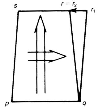
Before we proceed further, we examine the geometrical meaning of these tensors. We consider the Riemann tensor first. A crucial observation is that if we parallel transport a vector $V$ at $p$ to $q$ along two different curves $C$ and $C^{\prime }$ , the resulting vectors at $q$ are different in general (figure 7.2). If, however, we parallel transport a vector in a Euclidean space, where the parallel transport is defined in our usual sense, the resulting vector does not depend on the path along which it has been parallel transported. We expect that this non-integrability of parallel transport characterizes the intrinsic notion of curvature, which does not depend

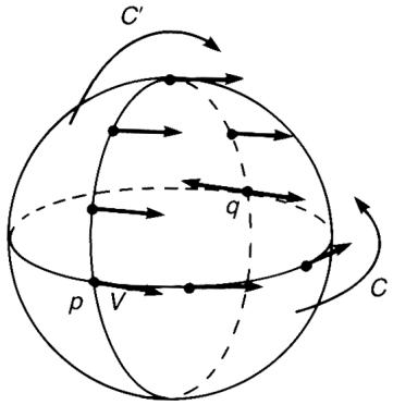
Figure 7.2. It is natural to define $V$ parallel transported along a great circle if the angle $V$ makes with the great circle is kept fixed. If $V$ at $p$ is parallel transported along great circles $C$ and $C^{\prime }$ , the resulting vectors at $q$ point in opposite directions.

on the special coordinates chosen. Let us take an infinitesimal parallelogram $pqs$ whose coordinates are $\{x^{\mu }\}$ , $\{x^{\mu }+{\epsilon }^{\mu }\}$ , $\{x^{\mu }+{\epsilon }^{\mu }+{\delta }^{\mu }\}$ and $\{x^{\mu }+{\delta }^{\mu }\}$ respectively, ${\epsilon }^{\mu }$ and ${\delta }^{\mu }$ being infinitesimal (figure 7.3). If we parallel transport a vector $V_0\in T_{p}M$ along $C=pqr$ , we will have a vector $V_C(r)\in T_{r}M$ . The vector $V_0$ parallel transported to $q$ along $C$ is

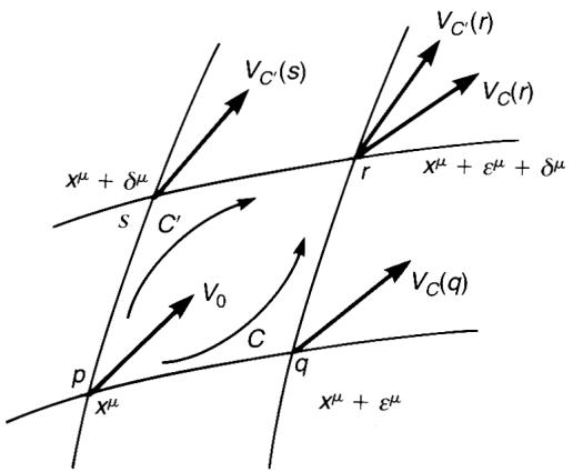
Figure 7.3. A vector $V_0$ at $p$ is parallel transported along $C$ and $C^{\prime }$ to yield $V_C(r)$ and $V_{C^{\prime }}(r)$ at $r$ . The curvature measures the difference between two vectors.

$$V_C^{\mu }(q)=V_0^{\mu }-V_0^{\kappa }{\Gamma }_{v\kappa }^{\mu }(p){\epsilon }^v.$$

Then $V_C^{\mu }(r)$ is given by

$$\begin{array}{rl}& V_C^{\mu }(r)=V_C^{\mu }(q)-V_C^{\kappa }(q){\Gamma }_{\nu \kappa }^{\mu }(q){\delta }^{\nu }\\ & =V_0^{\mu }-V_0^{\kappa }{\Gamma }_{v\kappa }^{\mu }{\epsilon }^v-\left[V_0^{\kappa }-V_0^{\rho }{\Gamma }_{\zeta \rho }^{\kappa }(p){\epsilon }^{\zeta }\right]\\ & \times \left[{\Gamma }_{v\kappa }^{\mu }(p)+{\partial }_{\lambda }{\Gamma }_{v\kappa }^{\mu }(p){\epsilon }^{\lambda }\right]{\delta }^{\nu }\\ & \simeq V_0^{\mu }-V_0^{\kappa }{\Gamma }_{v\kappa }^{\mu }(p){\epsilon }^v-V_0^{\kappa }{\Gamma }_{v\kappa }^{\mu }(p){\delta }^v\\ & -V_0^{\kappa }\left[{\partial }_{\lambda }{\Gamma }_{\nu \kappa }^{\mu }(p)-{\Gamma }_{\lambda \kappa }^{\rho }(p){\Gamma }_{\nu \rho }^{\mu }(p)\right]{\epsilon }^{\lambda }{\delta }^{\nu }\end{array}$$

where we have kept terms of up to order two in $\epsilon$ and $\delta$ . Similarly, parallel transport of $V_0$ along $C^{\prime }=psr$ yields another vector $V_{C^{\prime }}(r)\in T_{r}M$ , given by

$$\begin{array}{rl}& V_{C^{\prime }}^{\mu }(r)\simeq V_0^{\mu }-V_0^{\kappa }{\Gamma }_{\nu \kappa }^{\mu }(p){\delta }^{\nu }-V_0^{\kappa }{\Gamma }_{\nu \kappa }^{\mu }(p){\epsilon }^{\nu }\\ & -V_0^{\kappa }\left[{\partial }_{\nu }{\Gamma }_{\lambda \kappa }^{\mu }(p)-{\Gamma }_{\nu \kappa }^{\rho }(p){\Gamma }_{\lambda \rho }^{\mu }(p)\right]{\epsilon }^{\lambda }{\delta }^{\nu }.\end{array}$$

The two vectors at $r$ differ by

$$\begin{array}{rl}& V_{C^{\prime }}(r)-V_C(r)=V_0^{\kappa }[{\partial }_{\lambda }{\Gamma }_{\nu \kappa }^{\mu }(p)-{\partial }_{\nu }{\Gamma }_{\lambda \kappa }^{\mu }(p)\\ & -{\Gamma }_{\lambda \kappa }^{\rho }(p){\Gamma }_{v\rho }^{\mu }(p)+{\Gamma }_{v\kappa }^{\rho }(p){\Gamma }_{\lambda \rho }^{\mu }(p)]{\epsilon }^{\lambda }{\delta }^v\\ & =V_0^{\kappa }{R}_{\kappa \lambda \nu }^{\mu }{\epsilon }^{\lambda }{\delta }^{\nu }.\end{array}\text{\hspace{1em}(7.44)}$$

We next look at the geometrical meaning of the torsion tensor. Let $p\in M$ be a point whose coordinates are $\{x^{\mu }\}$ . Let $X={\epsilon }^{\mu }{e}_{\mu }$ and $Y={\delta }^{\mu }{e}_{\mu }$ be infinitesimal vectors in $T_{p}M$ . If these vectors are regarded as small displacements, they define two points $q$ and $s$ near $p$ , whose coordinates are $\{x^{\mu }+{\epsilon }^{\mu }\}$ and $\{x^{\mu }+{\delta }^{\mu }\}$ respectively (figure 7.4). If we parallel transport $X$ along the line $ps$ , we obtain a vector $s{r}_1$ whose component is ${\epsilon }^{\mu }-{\epsilon }^{\lambda }{\Gamma }_{\nu \lambda }^{\mu }{\delta }^{\nu }$ . The displacement vector connecting $p$ and $r_1$ is

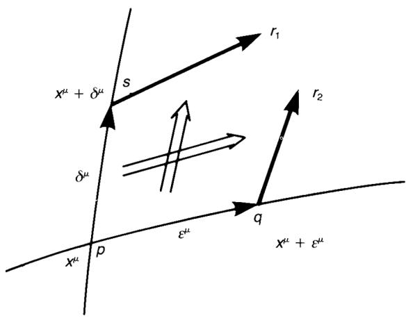
Figure 7.4. The vector $q{r}_2$ ( $s{r}_1$ ) is the vector $ps$ ( $pq$ ) parallel transported to $q$ ( $s$ ). In general, $r_1\ne r_2$ and the torsion measures the difference $r_2{r}_1$ .

$$p{r}_1=ps+s{r}_1={\delta }^{\mu }+{\epsilon }^{\mu }-{\Gamma }_{\nu \lambda }^{\mu }{\epsilon }^{\lambda }{\delta }^{\nu }.$$

Similarly, the parallel transport of ${\delta }^{\mu }$ along $pq$ yields a vector

$$p{r}_2=pq+q{r}_2={\epsilon }^{\mu }+{\delta }^{\mu }-{\Gamma }_{\lambda \nu }^{\mu }{\epsilon }^{\lambda }{\delta }^{\nu }.$$

In general, $r_1$ and $r_2$ do not agree and the difference is

$$r_2{r}_1=p{r}_2-p{r}_1=\left({\Gamma }_{\nu \lambda }^{\mu }-{\Gamma }_{\lambda \nu }^{\mu }\right){\epsilon }^{\lambda }{\delta }^{\nu }=T_{\nu \lambda }^{\mu }{\epsilon }^{\lambda }{\delta }^{\nu }.\text{\hspace{1em}(7.45)}$$

Thus, the torsion tensor measures the failure of the closure of the parallelogram made up of the small displacement vectors and their parallel transports.

Example 7.2

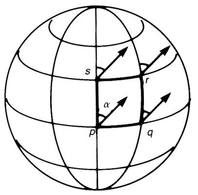
Suppose we are navigating on the surface of the Earth. We define a vector to be parallel transported if the angle between the vector and the latitude is kept fixed during the navigation. [Remarks: This definition of parallel transport is not the usual one. For example, the geodesic is not a great circle but a straight line on Mercator’s projection. See example 7.5.] Suppose we navigate along a small quadrilateral $pqs$ made up of latitudes and longitudes (figure 7.5(a)). We parallel transport a vector at $p$ along $pqr$ and $psr$ , separately. According to our definition of parallel transport, two vectors at $r$ should agree, hence the curvature tensor vanishes. To find the torsion, we parametrize the points $p,q,r$ and $s$ as in figure 7.5(b). We find the torsion by evaluating the difference between $p{r}_1$ and $p{r}_2$ as in (7.45). If we parallel transport the vector $pq$ along $ps$ , we obtain a vector $s{r}_1$ , whose length is $R\sin \theta \mathrm{d}\varphi$ . However, a parallel transport of the vector $ps$ along $pq$ yields a vector $q{r}_2=qr$ . Since $sr$ has a length $R\sin (\theta -\mathrm{d}\theta )\mathrm{d}\varphi \simeq R\sin \theta \mathrm{d}\varphi -R\cos \theta \mathrm{d}\theta \mathrm{d}\varphi$ , we find that $r_1{r}_2$ has a length $R\cos \theta \mathrm{d}\theta \mathrm{d}\varphi$ . Since $r_1{r}_2$ is parallel to $-\partial /\partial \varphi$ , the connection has a torsion $T_{\theta \varphi }^{\varphi }$ , see (7.45). From $g_{\varphi \varphi }=R^2{\sin }^2\theta$ , we find that $r_1{r}_2$ has components $(0,-\cot \theta \mathrm{d}\theta \mathrm{d}\varphi )$ . Since the $\varphi$ -component of $r_1{r}_2$ is equal to $T_{\theta \varphi }^{\varphi }\mathrm{d}\theta \mathrm{d}\varphi$ , we obtain $T_{\theta \varphi }^{\varphi }=-\cot \theta$ .

(a)

Figure 7.5. (a) If a vector makes an angle $\alpha$ with the longitude at $p$ , this angle is kept fixed during parallel transport. (b) The vector $s{r}_1(q{r}_2)$ is the vector $pq(ps)$ parallel transported to $s(q)$ . The torsion does not vanish.

Note that the basis $\{\partial /\partial \theta ,\partial /\partial \varphi \}$ is not well defined at the poles. It is known that the sphere $S^2$ does not admit two vector fields which are linearly independent everywhere on $S^2$ . Any vector field on $S^2$ must vanish somewhere on $S^2$ and

$$(\theta -\mathrm{d}\theta ,\varphi )(\theta -\mathrm{d}\theta ,\varphi +\mathrm{d}\varphi )$$

(b)

$(\theta ,\varphi )$

$(\theta ,\varphi +\mathsf{d}\varphi )$

hence cannot be linearly independent of the other vector field there. If an $m$ -dimensional manifold $M$ admits $m$ vector fields which are linearly independent everywhere, $M$ is said to be parallelizable. On a parallelizable manifold, we can use these $m$ vector fields to define a tangent space at each point of $M$ . A vector $V_p\in T_{p}M$ is defined to be parallel to $V_q\in T_{q}M$ if all the components of $V_p$ at $T_{p}M$ are equal to those of $V_q$ at $T_{q}M$ . Since the vector fields are defined throughout $M$ , this parallelism should be independent of the path connecting $p$ and $q$ , hence the Riemann curvature tensor vanishes although the torsion tensor may not in general. For $S^m$ , this is possible only when $m=1,3$ and 7, which is closely related to the existence of complex numbers, quaternions and octonions, respectively. For definiteness, let us consider

$$S^3=\left\{(x^1,x^2,x^3,x^4)|\sum _{i=1}^4(x^i{)}^2=1\right\}$$

embedded in $({\mathbb{R}}^4,\delta )$ . Three orthonormal vectors

$${\mathbf{e}}_1(\mathbf{x})=\left(-x^2,x^1,-x^4,x^3\right)$$

$${\mathbf{e}}_2(\mathbf{x})=\left(-x^3,x^4,x^1,-x^2\right)\text{\hspace{1em}(7.46)}$$

$${\mathbf{e}}_3(\mathbf{x})=\left(-x^4,-x^3,x^2,x^1\right)$$

are orthogonal to $x=(x^1,x^2,x^3,x^4)$ and linearly independent everywhere on $S^3$ , hence define the tangent space $T_x{S}^3$ . Two vectors $V_1(x)$ and $V_2(y)$

are parallel if $V_1(x)=\sum c^i{e}_i(x)$ and $V_2(y)=\sum c^i{e}_i(y)$ . The connection coefficients are computed from (7.14). Let $\epsilon e_1(x)$ be a small displacement under which $x=(x^1,x^2,x^3,x^4)$ changes to $x^{\prime }=x+\epsilon e_1(x)=\{x^1-\epsilon x^2,x^2+\epsilon x^1,x^3-\epsilon x^4,x^4+\epsilon x^3\}$ . The difference between the basis vectors at $x$ and $x^{\prime }$ is $e_2(x^{\prime })-e_2(x)=(-x^3-\epsilon x^4,x^4+\epsilon x^3,x^1-\epsilon x^2,-x^2-\epsilon x^1)-(-x^3,x^4,x^1,-x^2)=-\epsilon e_3(x)=\epsilon {\Gamma }_{12}^{\mu }{e}_{\mu }(x)$ , hence ${\Gamma }_{12}^3=-1,{\Gamma }_{12}^1={\Gamma }_{12}^2=0$ . Similarly, ${\Gamma }_{21}^3=1$ hence we find $T_{12}^3=-2$ . The reader should complete the computation of the connection coefficients and verify that $T_{\mu \nu }^{\lambda }=-2(+2)$ if $(\lambda \mu \nu )$ is an even (odd) permutation of (123) and vanishes otherwise.

Let us see how this parallelizability of $S^3$ is related to the existence of quaternions. The multiplication rule of quaternions is

$$\begin{array}{rl}& \left(x^1,x^2,x^3,x^4\right)\cdot \left(y^1,y^2,y^3,y^4\right)\\ & =(x^1{y}^1-x^2{y}^2-x^3{y}^3-x^4{y}^4,x^1{y}^2+x^2{y}^1+x^3{y}^4-x^4{y}^3,\\ & x^1{y}^3-x^2{y}^4+x^3{y}^1+x^4{y}^2,x^1{y}^4+x^2{y}^3-x^3{y}^2+x^4{y}^1).\end{array}\text{\hspace{1em}(7.47)}$$

$S^3$ may be defined by the set of unit quaternions

$$S^3=\left\{\left(x^1,x^2,x^3,x^4\right)\mid \mathbf{x}\cdot \bar{\mathbf{x}}=1\right\}$$

where the conjugate of $x$ is defined by $\bar{x}=(x^1,-x^2,-x^3,-x^4)$ . According to (7.46), the tangent space at $x_0=(1,0,0,0)$ is spanned by

$${\mathbf{e}}_1=(0,1,0,0){\mathbf{e}}_2=(0,0,1,0){\mathbf{e}}_3=(0,0,0,1).$$

Then the basis vectors (7.46) of the tangent space at $\mathbf{x}=(x^1,x^2,x^3,x^4)$ are expressed as the quaternion products

$${\mathbf{e}}_1(\mathbf{x})={\mathbf{e}}_1\cdot \mathbf{x}{\mathbf{e}}_2(\mathbf{x})={\mathbf{e}}_2\cdot \mathbf{x}{\mathbf{e}}_3(\mathbf{x})={\mathbf{e}}_3\cdot \mathbf{x}.\text{\hspace{1em}(7.48)}$$

Because of this algebra, it is always possible to give a set of basis vectors at an arbitrary point of $S^3$ once it is given at some point, $x_0=(1,0,0,0)$ , for example.

By the same token, a Lie group is parallelizable. If the set of basis vectors $\{V_1,\dots ,V_m\}$ at the unit element $e$ of a Lie group $G$ is given, we can always find a set of basis vectors of $T_{g}G$ by the left translation of $\{V_{\mu }\}$ (see section 5.6),

$$\left\{V_1,\dots ,V_n\right\}\stackrel{L_{g\ast }}{\to }\left\{X_1{|}_g,\dots ,X_n{|}_g\right\}.\text{\hspace{1em}(7.49)}$$

7.3.3 The Ricci tensor and the scalar curvature

From the Riemann curvature tensor, we construct new tensors by contracting the indices. The Ricci tensor $Ric$ is a type $(0,2)$ tensor defined by

$$Ric(X,Y)\equiv ⟨\mathrm{d}{x}^{\mu },R\left(e_{\mu },Y\right)X⟩\text{\hspace{1em}(7.50a)}$$

whose component is

$$Ri{c}_{\mu v}=Ric\left(e_{\mu },e_v\right)=R_{\mu \lambda v}^{\lambda }.\text{\hspace{1em}(7.50b)}$$

The scalar curvature $\mathcal{R}$ is obtained by further contracting indices,

$$\mathcal{R}\equiv g^{\mu v}Ric\left(e_{\mu },e_v\right)=g^{\mu v}Ri{c}_{\mu v}.\text{\hspace{1em}(7.51)}$$

来源与版本

正文：英文 · OCR 机器稿 · 待校对

核对状态：OCR 机器稿 · 待校对

原书 PDF

来源版本：second-edition-local

来源 PDF SHA-256：fcd24c3371d092a8c699ccf5cf0765462924b6c48412804231076e8084b1940d

OCR 来源 SHA-256：0b6324f01172a3548cd34382e82fd8bfae574602b6b2cfaa357ba96bc2c35478

OCR 产物 SHA-256：e4fb984b3acf5d31ae8c08d512e8e25794c4a660db00c48713c5e43848ec72e2