10.5 Gauge theories

As we have remarked several times, a gauge potential can be regarded as a local expression for a connection in a principal bundle. The Yang-Mills field strength is then identified with the local form of the curvature associated with the connection. We summarize here the relevant aspects of gauge theories from the geometrical viewpoint.

10.5.1 U(1) gauge theory

Maxwell’s theory of electromagnetism is described by the U(1) gauge group. U(1) is Abelian and one dimensional, hence we omit all the group indices $\alpha ,\beta ,\dots$ and put the structure constants $f_{\alpha \beta }^{\gamma }=0$ . Suppose the base space $M$ is a four-dimensional Minkowski spacetime. From corollary 9.1, we find that the U(1) bundle $P$ is trivial, namely $P={\mathbb{R}}^4\times \mathrm{U}(1)$ and a single local trivialization over $M$ is required. The gauge potential is simply

$$\mathcal{A}={\mathcal{A}}_{\mu }\mathrm{d}{x}^{\mu }.\text{\hspace{1em}(10.81)}$$

Our gauge potential $\mathcal{A}$ differs from the usual vector potential $A$ by the Lie algebra factor $\mathrm{i}:{\mathcal{A}}_{\mu }=\mathrm{i}{A}_{\mu }$ . The field strength is

$$\mathcal{F}=\mathrm{d}\mathcal{A}.\text{\hspace{1em}(10.82a)}$$

In components, we have

$${\mathfrak{F}}_{\mu v}=\partial {\mathcal{A}}_v/\partial x^{\mu }-\partial {\mathcal{A}}_{\mu }/\partial x^v.\text{\hspace{1em}(10.82b)}$$

$\mathcal{F}$ satisfies the Bianchi identity,

$$\mathrm{d}\mathcal{F}=\mathcal{F}\wedge \mathcal{A}-\mathcal{A}\wedge \mathcal{F}=0.\text{\hspace{1em}(10.83a)}$$

This should be expected from the outset since $\mathcal{F}$ is exact, $\mathcal{F}=\mathrm{d}\mathcal{A}$ ; and hence closed, $\mathrm{d}\mathcal{F}={\mathrm{d}}^2\mathcal{A}=0$ . In components, we have

$${\partial }_{\lambda }{\mathcal{F}}_{\mu v}+{\partial }_v{\mathcal{F}}_{\lambda \mu }+{\partial }_{\mu }{\mathcal{F}}_{v\lambda }=0.\text{\hspace{1em}(10.83b)}$$

If we identify the components ${\mathcal{F}}_{\mu \nu }\equiv \mathrm{i}{F}_{\mu \nu }$ with the electric field $E$ and the magnetic field $B$ as

$$E_i=F_{i0},B_i=\frac{1}{2}{ϵ}_{ijk}{F}_{jk}(i,j,k=1,2,3)\text{\hspace{1em}(10.84)}$$

(10.83b) reduces to two of Maxwell’s equations,

$$\nabla \times \mathbf{E}+\frac{\partial \mathbf{B}}{\partial t}=0\nabla \cdot \mathbf{B}=0.\text{\hspace{1em}(10.83c)}$$

These equations are geometrical rather than dynamical. To find the dynamics, we have to specify the action. The Maxwell action $S_{\mathrm{M}}[\mathcal{A}]$ is a functional of $\mathcal{A}$ and is given by

$${\mathcal{S}}_{\mathrm{M}}[\mathcal{A}]\equiv \frac{1}{4}{\int }_{{\mathbb{R}}^4}{\mathcal{F}}_{\mu v}{\mathcal{F}}^{\mu v}{\mathrm{d}}^{4}x=-\frac{1}{4}{\int }_{{\mathbb{R}}^4}{F}_{\mu v}{F}^{\mu v}{\mathrm{d}}^{4}x.\text{\hspace{1em}(10.85a)}$$

Exercise 10.12

(a) Let $\ast {\mathcal{F}}_{\mu \nu }\equiv \frac{1}{2}{\mathcal{F}}^{\kappa \lambda }{\epsilon }_{\kappa \lambda \mu \nu }$ be the dual of ${\mathcal{F}}_{\mu \nu }$ . Show that

$${\mathcal{S}}_{\mathrm{M}}[\mathcal{A}]=-\frac{1}{4}{\int }_{{\mathbb{R}}^4}\mathcal{F}\wedge \ast \mathcal{F}.\text{\hspace{1em}(10.85b)}$$

(b) Use (10.84) to show that

$$-\frac{1}{4}{F}_{\mu v}{F}^{\mu v}=\frac{1}{2}\left({\mathbf{E}}^2-{\mathbf{B}}^2\right).\text{\hspace{1em}(10.86)}$$

Show also that

$$F_{\mu v}\ast F^{\mu v}=\mathbf{B}\cdot \mathbf{E}.\text{\hspace{1em}(10.87)}$$

By the variation of $S_{\mathrm{M}}[\mathcal{A}]$ with respect to ${\mathcal{A}}_{\mu }$ , we obtain the equation of motion,

$${\partial }_{\mu }{\mathcal{F}}^{\mu v}=0.\text{\hspace{1em}(10.88a)}$$

We find this equation is reduced to the second set of Maxwell’s equations (in the vacuum):

$$\nabla \cdot \mathbf{E}=0\nabla \times \mathbf{B}-\frac{\partial \mathbf{E}}{\partial t}=0.\text{\hspace{1em}(10.88b)}$$

10.5.2 The Dirac magnetic monopole

We have studied Maxwell’s theory of electromagnetism defined on ${\mathbb{R}}^4$ . The triviality of the base space makes the U(1) bundle trivial. Poincaré’s lemma ensures that the field strength $\mathcal{F}$ is globally exact: $\mathcal{F}=\mathrm{d}\mathcal{A}$ . It is interesting to extend our analysis to U(1) bundles over a non-trivial base space. We assume everything is independent of time for simplicity.

The Dirac monopole is defined in ${\mathbb{R}}^3$ with the origin O removed. ${\mathbb{R}}^3-\{0\}$ and $S^2$ are of the same homotopy type and the relevant bundle is a U(1) bundle $P(S^2,\mathrm{U}(1))$ . $S^2$ is covered by two charts

$$U_{\mathrm{N}}\equiv \{(\theta ,\varphi )|0\le \theta \le \frac{1}{2}\pi +ϵ\}{U}_{\mathrm{S}}\equiv \{(\theta ,\varphi )|\frac{1}{2}\pi -ϵ\le \theta \le \pi \}$$

where $\theta$ and $\varphi$ are polar coordinates. Let $\omega$ be an Ehresmann connection on $P$ . Take a local section ${\sigma }_{\mathrm{N}}({\sigma }_{\mathrm{S}})$ on $U_{\mathrm{N}}(U_{\mathrm{S}})$ and define the local gauge potentials

$${\mathcal{A}}_{\mathrm{N}}={\sigma }_{\mathrm{N}}^{\ast }\omega {\mathcal{A}}_{\mathrm{S}}={\sigma }_{\mathrm{S}}^{\ast }\omega .$$

We take ${\mathcal{A}}_{\mathrm{N}}$ and ${\mathcal{A}}_{\mathrm{S}}$ to be of the Wu-Yang form (section 1.9),

$${\mathcal{A}}_{\mathrm{N}}=\mathrm{i}g(1-\cos \theta )\mathrm{d}\varphi {\mathcal{A}}_{\mathrm{S}}=-\mathrm{i}g(1+\cos \theta )\mathrm{d}\varphi \text{\hspace{1em}(10.89)}$$

where $g$ is the strength of the monopole.

Let $t_{\mathrm{NS}}$ be the transition function defined on the equator $U_{\mathrm{N}}\cap U_{\mathrm{S}}$ . $t_{\mathrm{NS}}$ defines a map from $S^1$ (equator) to $\mathrm{U}(1)$ (structure group), which is classified by ${\pi }_1(\mathrm{U}(1))=\mathbb{Z}$ , see example 9.7. Let us write

$$t_{\mathrm{NS}}(\varphi )=\exp [\mathrm{i}\phi (\varphi )](\phi :S^1\to \mathbb{R}).\text{\hspace{1em}(10.90)}$$

The gauge potentials ${\mathcal{A}}_{\mathrm{N}}$ and ${\mathcal{A}}_{\mathrm{S}}$ are related on $U_{\mathrm{N}}\cap U_{\mathrm{S}}$ by

$${\mathcal{A}}_{\mathrm{N}}=t_{\mathrm{NS}}^{-1}{\mathcal{A}}_{\mathrm{S}}{t}_{\mathrm{NS}}+t_{\mathrm{NS}}^{-1}\mathrm{d}{t}_{\mathrm{NS}}={\mathcal{A}}_{\mathrm{S}}+\mathrm{id}\phi .\text{\hspace{1em}(10.91)}$$

For the gauge potentials (10.89), we find

$$\mathrm{d}\phi =-\mathrm{i}\left({\mathcal{A}}_{\mathrm{N}}-{\mathcal{A}}_{\mathrm{S}}\right)=2g\mathrm{d}\varphi .$$

While $\varphi$ runs from 0 to $2\pi$ around the equator, $\phi (\varphi )$ takes the range

$$\Delta \phi \equiv \int \mathrm{d}\phi ={\int }_0^{2\pi }2g\mathrm{d}\varphi =4\pi g.\text{\hspace{1em}(10.92)}$$

For $t_{\mathrm{NS}}$ to be defined uniquely, $\Delta \phi$ must be a multiple of $2\pi$

$$\Delta \phi /2\pi =2g\in \mathbb{Z}\text{\hspace{1em}(10.93)}$$

which is the quantization condition of the magnetic monopole. The integer $2g$ represents the homotopy class to which this bundle belongs. This number is also obtained by considering $F_{\mathrm{N}}=\mathrm{d}{A}_{\mathrm{N}}$ and $F_{\mathrm{S}}=\mathrm{d}{A}_{\mathrm{S}}$ ( ${\mathcal{F}}_{\mathrm{N}}=\mathrm{i}{F}_{\mathrm{N}}$ etc). The total flux $\Phi$ is

$$\begin{array}{rl}\mathbf{\Phi }& ={\int }_{S^2}\mathbf{B}\cdot \mathrm{d}\mathbf{S}={\int }_{U_{\mathrm{N}}}\mathrm{d}{A}_{\mathrm{N}}+{\int }_{U_{\mathrm{S}}}\mathrm{d}{A}_{\mathrm{S}}\\ & ={\int }_{S^1}{A}_{\mathrm{N}}-{\int }_{S^1}{A}_{\mathrm{S}}=2g{\int }_0^{2\pi }\mathrm{d}\varphi =4\pi g.\end{array}\text{\hspace{1em}(10.94)}$$

Thus, the curvature, that is the pair of the field strengths $\mathrm{d}{A}_{\mathrm{N}}$ and $\mathrm{d}{A}_{\mathrm{S}}$ , characterizes the twisting of the bundle. We discuss this further in chapter 11.

10.5.3 The Aharonov-Bohm effect

In the elementary study of electromagnetism, the electric and magnetic fields (that is $F_{\mu \nu }$ ) are of central interest. The vector potential $A$ and the scalar potential $\varphi =A_0$ are considered to be of secondary importance. In quantum mechanics, however, there are a variety of situations in which $F_{\mu \nu }$ are not sufficient to describe the phenomena and the use of $A_{\mu }=(A,A_0)$ is essential. One of these examples is the Aharonov-Bohm effect.

The Aharonov-Bohm (AB) experiment is schematically described in figure 10.4. A beam of electrons with charge $e$ is incoming from the far left and forms an interference pattern on the screen C. A solenoid of infinite length is placed in the middle of the beam. A shield S prevents electrons from penetrating into the solenoid. Accordingly, the electrons do not feel the magnetic field at all. What about the gauge field $A_{\mu }$ ?

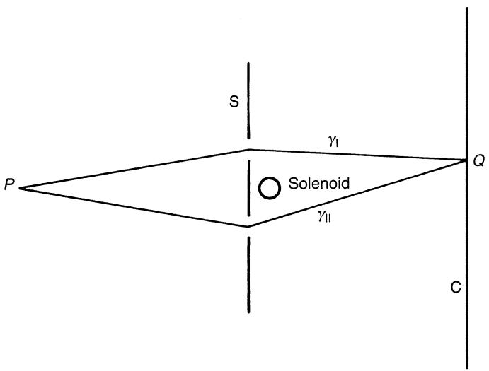
Figure 10.4. The Aharonov-Bohm experiment. $B=0$ outside the solenoid.

For simplicity, we make the radius of the solenoid infinitesimally small, keeping the total flux $\Phi ={\int }_S\mathbf{B}\cdot \mathrm{d}\mathbf{S}$ fixed. It is easy to verify that

$$\mathbf{A}(\mathbf{r})=\left(-\frac{y\Phi }{2\pi r^2},\frac{x\Phi }{2\pi r^2},0\right)A_0=0\text{\hspace{1em}(10.95)}$$

satisfies $\int (\nabla \times \mathbf{A})\cdot \mathrm{d}\mathbf{S}=\Phi$ and $\nabla \times \mathbf{A}=0$ for $r\ne 0$ . The vector potential does not vanish outside the solenoid. Classically, the solenoid cannot have any influence on electrons since the Lorentz force $e(v\times B)$ vanishes on the path of the beam.

In quantum mechanics, the Hamiltonian $H$ of this system is

$$\mathcal{H}=-\frac{1}{2m}{\left(\frac{\partial }{\partial x^{\mu }}-\mathrm{i}e{A}_{\mu }\right)}^2+V(\mathbf{r})\text{\hspace{1em}(10.96)}$$

where $V(\mathbf{r})$ represents the effect of the experimental apparatus. Semiclassically, we can distinguish between the paths ${\gamma }_{\mathrm{I}}$ and ${\gamma }_{\mathrm{II}}$ in figure 10.4. We write the wavefunction corresponding to ${\gamma }_{\mathrm{I}}({\gamma }_{\mathrm{II}})$ as ${\psi }_{\mathrm{I}}({\psi }_{\mathrm{II}})$ when $A=0$ . If $A\ne 0$ , the wavefunction is given by the gauge-transformed form,

$${\psi }_i^{\mathbf{A}}(\mathbf{r})\equiv \exp \left(\mathrm{i}e{\int }_P^{\mathbf{r}}\mathbf{A}\left({\mathbf{r}}^{\prime }\right)\cdot \mathrm{d}{\mathbf{r}}^{\prime }\right){\psi }_i(\mathbf{r})(i=\mathrm{I},\mathrm{II})\text{\hspace{1em}(10.97)}$$

where $P$ is a reference point far from the apparatus. Let us consider a superposition ${\psi }_{\mathrm{I}}^A+{\psi }_{\mathrm{II}}^A$ of wavefunctions ${\psi }_{\mathrm{I}}^A$ and ${\psi }_{\mathrm{II}}^A$ such that ${\psi }_{\mathrm{I}}^A(P)={\psi }_{\mathrm{II}}^A(P)$ . Its amplitude at a point $Q$ on the screen is

$$\begin{array}{rl}& {\psi }_{\mathrm{I}}^{\mathbf{A}}(\mathbf{Q})+{\psi }_{\mathrm{II}}^{\mathbf{A}}(\mathbf{Q})=\exp \left(\mathrm{i}e{\int }_{{\gamma }_{\mathrm{I}}}\mathbf{A}({\mathbf{r}}^{\prime })\cdot \mathrm{d}{\mathbf{r}}^{\prime }\right){\psi }_{\mathrm{I}}(\mathbf{Q})\\ & +\exp \left(\mathrm{i}e{\int }_{{\gamma }_{\mathrm{II}}}\mathbf{A}\left({\mathbf{r}}^{\prime }\right)\cdot \mathrm{d}{\mathbf{r}}^{\prime }\right){\psi }_{\mathrm{II}}(Q)\\ & =\exp \left(\mathrm{i}e{\int }_{{\gamma }_{\mathrm{II}}}\mathbf{A}\cdot \mathrm{d}{\mathbf{r}}^{\prime }\right)\left[\exp \left(\mathrm{i}e{\oint }_{\gamma }\mathbf{A}\cdot \mathrm{d}{\mathbf{r}}^{\prime }\right){\psi }_{\mathrm{I}}(Q)+{\psi }_{\mathrm{II}}(Q)\right]\end{array}\text{\hspace{1em}(10.98)}$$

where $\gamma \equiv {\gamma }_{\mathrm{I}}-{\gamma }_{\mathrm{II}}$ . It is evident that even though $B=0$ at the points in space through which the electrons travel, the wavefunction depends on the vector potential $A$ . From Stokes’ theorem, we find that

$${\oint }_{\gamma }\mathbf{A}\cdot \mathrm{d}{\mathbf{r}}^{\prime }={\int }_S(\nabla \times \mathbf{A})\cdot \mathrm{d}S={\int }_S\mathbf{B}\cdot \mathrm{d}S=\Phi \text{\hspace{1em}(10.99)}$$

where $S$ is a surface bounded by $\gamma$ . From this and (10.98), we find the interference pattern should be the same for two values of the fluxes ${\Phi }_{\mathrm{a}}$ and ${\Phi }_{\mathrm{b}}$ if

$$e\left({\Phi }_{\mathrm{a}}-{\Phi }_{\mathrm{b}}\right)=2\pi nn\in \mathbb{Z}.\text{\hspace{1em}(10.100)}$$

What is the geometry underlying the Aharonov-Bohm effect? Since the problem is essentially two dimensional, we consider a region $M={\mathbb{R}}^2-\{0\}$ , where the solenoid is assumed to be at the origin. The relevant bundles are the principal bundle $P(M,\mathrm{U}(1))$ and its associated bundle $E=P{\times }_{\rho }\mathbb{C}$ , where $\mathrm{U}(1)$ acts on $\mathbb{C}$ in an obvious way. The bundle $E$ is a complex line bundle over $M$ , whose section is a wavefunction $\psi$ .

Let us define a Lie-algebra-valued one-form $\mathcal{A}=\mathrm{i}A=\mathrm{i}{A}_{\mu }\mathrm{d}{x}^{\mu }$ . The covariant derivative associated with this local connection is $\mathcal{D}=\mathrm{d}+\mathcal{A}$ , where

$\mathcal{A}$ is given by (10.95). Since $\mathrm{d}\mathcal{A}=\mathcal{F}=0$ , this connection is locally flat. Let us consider the unit circle $S^1$ which encloses the solenoid at the origin. We parametrize $S^1$ as ${\mathrm{e}}^{\mathrm{i}\theta }$ ( $0\le \theta \le 2\pi$ ) and write the connection on $S^1$ as

$$\mathcal{A}=\mathrm{i}\frac{\Phi }{2\pi }\mathrm{d}\theta .\text{\hspace{1em}(10.101)}$$

This is obtained from (10.95) by putting $r=1$ . We require that the wavefunction $\psi$ be parallel transported along $S^1$ with respect to this local connection, namely

$$\mathcal{D}\psi (\theta )=\left(\mathrm{d}+\mathrm{i}\frac{\Phi }{2\pi }\mathrm{d}\theta \right)\psi (\theta )=0.\text{\hspace{1em}(10.102)}$$

The solution of (10.102) is easily found to be

$$\psi (\theta )={\mathrm{e}}^{-\mathrm{i}\Phi \theta /2\pi }.\text{\hspace{1em}(10.103)}$$

Taking this section $\psi$ amounts to neglecting the velocity of the electrons. The holonomy $\Gamma :{\pi }^{-1}(\theta =0)\to {\pi }^{-1}(\theta =2\pi )={\pi }^{-1}(\theta =0)$ is found to be

$$\Gamma :\psi (0)⟼{\mathrm{e}}^{-\mathrm{i}\Phi }\psi (0).\text{\hspace{1em}(10.104)}$$

In an experiment, a toroidal permalloy (20% Fe and 80% Ni) has been used to eliminate the edge effects (Tonomura et al 1983). The dimensions of the permalloy are several microns and it is coated with gold to prevent electrons from penetrating into the magnetic field.

10.5.4 Yang-Mills theory

Let us consider $\mathrm{SU}(2)$ gauge theory defined on ${\mathbb{R}}^4$ . The bundle which describes this gauge theory is $P({\mathbb{R}}^4,\mathrm{SU}(2))$ . Since ${\mathbb{R}}^4$ is contractible, there is just a single gauge potential

$$\mathcal{A}=A_{\mu }^{\alpha }{T}_{\alpha }\mathrm{d}{x}^{\mu }\text{\hspace{1em}(10.105)}$$

where $T_{\alpha }\equiv {\sigma }_{\alpha }/2\mathrm{i}$ generate the algebra $\mathfrak{su}(2)$

$$[T_{\alpha },T_{\beta }]={ϵ}_{\alpha \beta \gamma }{T}_{\gamma }.$$

The field strength is

$$\mathcal{F}\equiv \mathrm{d}\mathcal{A}+\mathcal{A}\wedge \mathcal{A}=\frac{1}{2}{\mathcal{F}}_{\mu \nu }\mathrm{d}{x}^{\mu }\wedge \mathrm{d}{x}^{\nu }\text{\hspace{1em}(10.106a)}$$

where

$${\mathcal{F}}_{\mu v}={\partial }_{\mu }{\mathcal{A}}_v-{\partial }_v{\mathcal{A}}_{\mu }+\left[{\mathcal{A}}_{\mu },{\mathcal{A}}_v\right]=F_{\mu v}^{\alpha }{T}_{\alpha }\text{\hspace{1em}(10.106b)}$$

$$F_{\mu v}^{\alpha }={\partial }_{\mu }{A}_{v\alpha }-{\partial }_v{A}_{\mu \alpha }+{ϵ}_{\alpha \beta \gamma }{A}_{\mu \beta }{A}_{v\gamma }.\text{\hspace{1em}(10.106c)}$$

The Bianchi identity is

$$\mathcal{D}\mathcal{F}=\mathrm{d}\mathcal{F}+[\mathcal{A},\mathcal{F}]=0.\text{\hspace{1em}(10.107)}$$

The Yang-Mills action is

$${\mathcal{S}}_{\mathrm{YM}}[\mathcal{A}]\equiv -\frac{1}{4}{\int }_M\mathrm{tr}\left({\mathcal{F}}_{\mu v}{\mathcal{F}}^{\mu v}\right)=\frac{1}{2}{\int }_M\mathrm{tr}(\mathcal{F}\wedge \ast \mathcal{F}).\text{\hspace{1em}(10.108)}$$

The variation with respect to ${\mathcal{A}}_{\mu }$ yields

$${\mathcal{D}}_{\mu }{\mathcal{F}}^{\mu v}=0\text{o r}\mathcal{D}\ast \mathcal{F}=0.\text{\hspace{1em}(10.109)}$$

10.5.5 Instantons

A path integral is well defined only on a space with a Euclidean metric. To evaluate this integral, it is important to find the local minima of the Euclidean action and compute the quantum fluctuations around them. Let us consider the SU(2) gauge theory on a four-dimensional Euclidean space ${\mathbb{R}}^4$ . The local minima of this theory are known as instantons (or pseudoparticles, Belavin et al (1975)), see section 1.10. It is easy to verify that the Euclidean action is

$${\mathcal{S}}_{\mathrm{YM}}^{\mathrm{E}}[\mathcal{A}]=\frac{1}{4}{\int }_M\mathrm{tr}\left({\mathcal{F}}_{\mu v}{\mathcal{F}}^{\mu v}\right)=-\frac{1}{2}{\int }_M\mathrm{tr}\left(\mathcal{F}\wedge \ast \mathcal{F}\right)\text{\hspace{1em}(10.110)}$$

where the Hodge $\ast$ is taken with respect to the Euclidean metric. As has been shown in section 1.10 the field strength corresponding to instantons is self-dual (anti-self-dual),

$${\mathcal{F}}_{\mu v}=\pm \ast {\mathcal{F}}_{\mu v}.\text{\hspace{1em}(10.111)}$$

The action of a self-dual (anti-self-dual) field configuration is

$${\mathcal{S}}_{\mathrm{YM}}^{\mathrm{E}}[\mathcal{A}]=-\frac{1}{2}{\int }_M\mathrm{tr}(\mathcal{F}\wedge \ast \mathcal{F})=\mp \frac{1}{2}{\int }_M\mathrm{tr}(\mathcal{F}\wedge \mathcal{F}).\text{\hspace{1em}(10.112)}$$

Let us consider the topological properties of an instanton. We require that

$${\mathcal{A}}_{\mu }(x)\to g(x{)}^{-1}{\partial }_{\mu }g(x)\text{a s}|x|\to L\text{\hspace{1em}(10.113)}$$

for the action to be finite, where $L$ is an arbitrary positive number. Since $|x|=L$ is the sphere $S^3$ , (10.113) defines a map $g:S^3\to \mathrm{SU}(2)$ which is classified by ${\pi }_3(\mathrm{SU}(2))\cong \mathbb{Z}$ . How is this reflected upon the transition function? We compactify ${\mathbb{R}}^4$ by adding the infinity. We suppose the South Pole of $S^4$ represents the points at infinity and the North Pole the origin. Under this compactification, we separate ${\mathbb{R}}^4$ into two pieces and identify them with the southern hemisphere $U_{\mathrm{S}}$ and the northern hemisphere $U_{\mathrm{N}}$ of $S^4$ as

$$U_{\mathrm{N}}=\{x\in {\mathbb{R}}^4||x|\le L+\epsilon \}\text{\hspace{1em}(10.114a)}$$

$$U_{\mathrm{S}}=\{x\in {\mathbb{R}}^4||x|\ge L-\epsilon \}\text{\hspace{1em}(10.114b)}$$

see figure 10.5. We assume there is no ‘twist’ of the gauge potential on $U_{\mathrm{S}}$ and choose

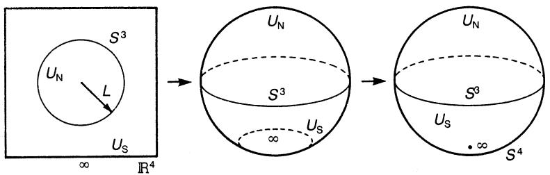
Figure 10.5. One-point compactification of ${\mathbb{R}}^4$ to $S^4$ .

$${\mathcal{A}}_{\mathrm{S}}(x)\equiv 0x\in U_{\mathrm{S}}.\text{\hspace{1em}(10.115)}$$

Then all the topological information about the bundle is contained in ${\mathcal{A}}_{\mathrm{N}}(x)$ or the transition function $t_{\mathrm{NS}}(x)$ on the ‘equator’ $S^3$ ( $=U_{\mathrm{N}}\cap U_{\mathrm{S}}$ ). Since ${\mathcal{A}}_{\mathrm{S}}=0$ , we have, for $x\in U_{\mathrm{N}}\cap U_{\mathrm{S}}$ ,

$${\mathcal{A}}_{\mathrm{N}}=t_{\mathrm{NS}}^{-1}{\mathcal{A}}_{\mathrm{S}}{t}_{\mathrm{NS}}+t_{\mathrm{NS}}^{-1}\mathrm{d}{t}_{\mathrm{NS}}=t_{\mathrm{NS}}^{-1}\mathrm{d}{t}_{\mathrm{NS}}.\text{\hspace{1em}(10.116)}$$

Thus, $g(x)$ in (10.113) is identified with the transition function $t_{\mathrm{NS}}(x)$ and classifying the maps $g:S^3\to \mathrm{SU}(2)$ amounts to classifying the transition functions according to ${\pi }_3(\mathrm{SU}(2))=\mathbb{Z}$ ; see example 9.11.

We now compute the degree of a map $g:S^3\to \mathrm{SU}(2)$ following Coleman (1979). First note that $\mathrm{SU}(2)\simeq S^3$ since

$$t^4{I}_2+t^i{\sigma }_i\in \mathrm{SU}(2)\leftrightarrow t^2+(t^4{)}^2=1.$$

Thus, maps $g:S^3\to \mathrm{SU}(2)$ are classified according to ${\pi }_3(\mathrm{SU}(2))\cong {\pi }_3(S^3)\cong \mathbb{Z}$ . We easily find the following.

(a) The constant map

$$g_0:x\in S^3\mapsto e\in \mathrm{SU}(2)\text{\hspace{1em}(10.117a)}$$

belongs to the class 0 (i.e. no winding) of ${\pi }_3(\mathrm{SU}(2))$ .

(b) The identity map (this is, in fact, the identity map $S^3\to S^3$ )

$$g_1:x\mapsto \frac{1}{r}\left[x^4{I}_2+x^i{\sigma }_i\right],r^2=x^2+(x^4{)}^2\text{\hspace{1em}(10.117b)}$$

defines the class 1 of ${\pi }_3(\mathrm{SU}(2))$ . The explicit form of the gauge potential corresponding to this homotopy class is given in section 1.10.

(c) The map

$$g_n\equiv (g_1{)}^n:x\mapsto r^{-n}{\left[x^4{I}_2+x^i{\sigma }_i\right]}^n\text{\hspace{1em}(10.117c)}$$

defines the class $n$ of ${\pi }_3(\mathrm{SU}(2))$ .

We recall that the strength (charge) of a magnetic monopole is given by the integral of the field strength $\mathcal{F}=\mathrm{d}\mathcal{A}$ over the sphere $S^2$ . We expect that a similar

relation exists for the instanton number. Since instantons are defined over $S^4$ , we have to find a four-form to be integrated over $S^4$ . A natural four-form is $\mathcal{F}\wedge \mathcal{F}$ . In the following, we shall omit the exterior product symbol when this does not cause confusion ( ${\mathcal{F}}^2$ stands for $\mathcal{F}\wedge \mathcal{F}$ ). Observe that $\mathrm{tr}{\mathcal{F}}^2$ is closed,

$$\begin{array}{rl}\mathrm{d}\mathrm{tr}{\mathcal{F}}^2& =\mathrm{tr}[\mathrm{d}\mathcal{FF}+\mathcal{F}\mathrm{d}\mathcal{F}]\\ & =\mathrm{tr}\{-[\mathcal{A},\mathcal{F}]\mathcal{F}-\mathcal{F}[\mathcal{A},\mathcal{F}]\}=0\end{array}\text{\hspace{1em}(10.118)}$$

where use has been made of the Bianchi identity $\mathrm{d}\mathcal{F}+[\mathcal{A},\mathcal{F}]=0$ . [Remarks: In the present case, (10.118) seems to be trivial since any four-form on $S^4$ is closed. Note, however, that (10.118) remains true even on higher-dimensional manifolds.] By Poincaré’s lemma, the closed form $\mathrm{tr}{\mathcal{F}}^2$ is locally exact,

$$\mathrm{tr}{\mathcal{F}}^2=\mathrm{d}K\text{\hspace{1em}(10.119)}$$

where $K$ is a local three-form. Thus, $\mathrm{tr}{\mathcal{F}}^2$ is an element of the de Rham cohomology group $H^4(S^4)$ . Later $\mathrm{tr}{\mathcal{F}}^2$ is identified with the second Chern character and $K$ its Chern-Simons form, see chapter 11.

Lemma 10.3

The three-form $K$ in (10.119) is given by

$$K=\mathrm{tr}\left[\mathcal{A}\mathrm{d}\mathcal{A}+\frac{2}{5}{\mathcal{A}}^3\right].\text{\hspace{1em}(10.120)}$$

Proof

A straightforward computation yields

$$\begin{array}{rl}& \mathrm{d}K=\mathrm{tr}\left[(\mathrm{d}\mathcal{A}{)}^2+\frac{2}{3}\left(\mathrm{d}\mathcal{A}{\mathcal{A}}^2-\mathcal{A}\mathrm{d}\mathcal{AA}+{\mathcal{A}}^2\mathrm{d}\mathcal{A}\right)\right]\\ & =\mathrm{tr}[(\mathcal{F}-{\mathcal{A}}^2)(\mathcal{F}-{\mathcal{A}}^2)\\ & +\frac{2}{3}\{(\mathcal{F}-{\mathcal{A}}^2){\mathcal{A}}^2-\mathcal{A}(\mathcal{F}-{\mathcal{A}}^2)\mathcal{A}+{\mathcal{A}}^2(\mathcal{F}-{\mathcal{A}}^2)\}]\\ & =\mathrm{tr}[{\mathcal{F}}^2-{\mathcal{A}}^2\mathcal{F}-\mathcal{F}{\mathcal{A}}^2+{\mathcal{A}}^4+\frac{2}{3}(\mathcal{F}{\mathcal{A}}^2-\mathcal{A}\mathcal{F}\mathcal{A}+{\mathcal{A}}^2\mathcal{F}-{\mathcal{A}}^4)]\end{array}$$

where use has been made of the identity $\mathrm{d}\mathcal{A}=\mathcal{F}-{\mathcal{A}}^2$ . Now we note that

$$\mathrm{tr}{\mathcal{A}}^4=0\mathrm{tr}\mathcal{A}\mathcal{F}\mathcal{A}=-\mathrm{tr}{\mathcal{A}}^2\mathcal{F}=-\mathrm{tr}\mathcal{F}{\mathcal{A}}^2.$$

For example, we have

$$\begin{array}{rl}\mathrm{tr}\mathcal{A}\mathcal{F}\mathcal{A}& =\frac{1}{2}\mathrm{tr}{\mathcal{A}}_{\kappa }{\mathcal{F}}_{\lambda \mu }{\mathcal{A}}_{\nu }d{x}^{\kappa }\wedge d{x}^{\lambda }\wedge d{x}^{\mu }\wedge d{x}^{\nu }\\ & =-\frac{1}{2}\mathrm{tr}{\mathcal{A}}_{\nu }{\mathcal{A}}_{\kappa }{\mathcal{F}}_{\lambda \mu }d{x}^{\nu }\wedge d{x}^{\kappa }\wedge d{x}^{\lambda }\wedge d{x}^{\mu }=-\mathrm{tr}{\mathcal{A}}^2\mathcal{F}\end{array}$$

where the cyclicity of the trace and the anti-commutativity of $\mathrm{d}{x}^{\mu }$ have been used. Then $\mathrm{d}K$ becomes

$$\begin{array}{rl}& \mathrm{d}K=\mathrm{tr}[{\mathcal{F}}^2-{\mathcal{A}}^2\mathcal{F}-\mathcal{F}{\mathcal{A}}^2+\frac{2}{3}\{\mathcal{F}{\mathcal{A}}^2+\frac{1}{2}(\mathcal{F}{\mathcal{A}}^2+{\mathcal{A}}^2\mathcal{F})+{\mathcal{A}}^2\mathcal{F}\}]\\ & \mathbf{\Sigma }=\mathrm{tr}{\mathcal{F}}^2\end{array}$$

as has been claimed.

$\square$

Lemma 10.4

Let $\mathcal{A}$ be the gauge potential of an instanton. Then it follows that

$${\int }_{S^4}\mathrm{tr}{\mathcal{F}}^2=-\frac{1}{3}{\int }_{S_3}\mathrm{tr}{\mathcal{A}}^3.\text{\hspace{1em}(10.121)}$$

Proof

From Stokes’ theorem, we find that

$${\int }_{U_{\mathrm{N}}}\mathrm{tr}{\mathcal{F}}^2={\int }_{U_{\mathrm{N}}}\mathrm{d}K={\int }_{S^3}K$$

where $U_{\mathrm{N}}$ is defined by (10.114) and $S^3=\partial U_{\mathrm{N}}$ . Since $\mathcal{F}=0$ on $S^3$ , we obtain

$$K=\mathrm{tr}[\mathcal{A}\mathrm{d}\mathcal{A}+\frac{2}{3}{\mathcal{A}}^3]=\mathrm{tr}[\mathcal{A}(\mathcal{F}-{\mathcal{A}}^2)+\frac{2}{3}{\mathcal{A}}^3]=-\frac{1}{3}\mathrm{tr}{\mathcal{A}}^3$$

on $S^3$ , from which we find that

$${\int }_{U_{\mathrm{N}}}\mathrm{tr}{\mathcal{F}}^2={\int }_{S^4}\mathrm{tr}{\mathcal{F}}^2=-\frac{1}{3}{\int }_{S^3}\mathrm{tr}{\mathcal{A}}^3$$

where we have added ${\int }_{U_S}\mathrm{tr}{\mathcal{F}}^2=0$ since ${\mathcal{A}}_S\equiv 0$

Note that $\mathrm{tr}{\mathcal{F}}^2$ is invariant under the gauge transformation,

$$\mathrm{tr}{\mathcal{F}}^2\to \mathrm{tr}\left[g^{-1}{\mathcal{F}}^{2}g\right]=\mathrm{tr}{\mathcal{F}}^2.$$

Thus, it is reasonable to assume that $\mathrm{tr}{\mathcal{F}}^2$ indeed contains a certain amount of topological information about the bundle, which is independent of particular connections. Let us consider the gauge fields (10.117a-c) given before. We find:

(a) For $g_0(x)\equiv e$ , we have $\mathcal{A}=0$ on $S^3$ . Since the bundle is trivial we may take $\mathcal{A}=0$ throughout $S^4$ . Then $\mathcal{F}=0$ , hence

$${\int }_{S^4}\mathrm{tr}{\mathcal{F}}^2=-\frac{1}{3}{\int }_{S^3}\mathrm{tr}{\mathcal{A}}^3=0.\text{\hspace{1em}(10.122)}$$

Note that this relation is true for any gauge potential which is obtained from $\mathcal{A}=0$ by smooth gauge transformations, that is for any gauge potential of the form $\mathcal{A}(x)=g(x{)}^{-1}\mathrm{d}g(x),x\in S^4$ .

(b) Next consider a gauge potential whose value on $S^3$ is given by (10.117b) as

$$\mathcal{A}=\frac{1}{r}\left(x^4-\mathrm{i}{x}^k{\sigma }_k\right)\mathrm{d}\left(\frac{1}{r}\left(x^4+\mathrm{i}{x}^l{\sigma }_l\right)\right).\text{\hspace{1em}(10.123)}$$

A considerable simplification is achieved if we note that the integrand $\mathrm{tr}{\mathcal{A}}^3$ should not depend on the point on $S^3$ at which it is evaluated since $g_1$ maps $S^3$ onto $\mathrm{SU}(2)\cong S^3$ in a uniform way. So we may evaluate it at the North Pole $(x^4=1,x=0)$ of the unit sphere. We then find $\mathcal{A}=\mathrm{i}{\sigma }_k\mathrm{d}{x}^k$ and

$$\begin{array}{rl}\mathrm{tr}{\mathcal{A}}^3& ={\mathrm{i}}^3\mathrm{tr}\left[{\sigma }_i{\sigma }_j{\sigma }_k\right]\mathrm{d}{x}^i\wedge \mathrm{d}{x}^j\wedge \mathrm{d}{x}^k\\ & =2{\epsilon }_{ijk}\mathrm{d}{x}^i\wedge \mathrm{d}{x}^j\wedge \mathrm{d}{x}^k=12\mathrm{d}{x}^1\wedge \mathrm{d}{x}^2\wedge \mathrm{d}{x}^3.\end{array}\text{\hspace{1em}(10.124)}$$

Next we note that $(x^1,x^2,x^3)$ is a good coordinate system on each hemisphere of $S^3$ and $\omega \equiv \mathrm{d}{x}^1\wedge \mathrm{d}{x}^2\wedge \mathrm{d}{x}^3$ is a volume element at the North Pole. We find

$${\int }_{S^3}\mathrm{tr}{\mathcal{A}}^3=12{\int }_{S^3}\omega =12(2{\pi }^2)=24{\pi }^2$$

where $2{\pi }^2$ is the area of the unit sphere $S^3$ . We finally obtain

$$-\frac{1}{8{\pi }^2}{\int }_{S^4}\mathrm{tr}{\mathcal{F}}^2=\frac{1}{24{\pi }^2}{\int }_{S^3}\mathrm{tr}{\mathcal{A}}^3=1.\text{\hspace{1em}(10.125)}$$

(c) Next we consider the map $g_n:S^3\to \mathrm{SU}(2)$ given by (10.117c). We show that $g_2=g_1{g}_1$ has a winding number 2. We divide $S^3$ into the northern hemisphere $U_{\mathrm{N}}^{(3)}$ and the southern hemisphere $U_{\mathrm{S}}^{(3)}$ . Given a map $g_1:S^3\to \mathrm{SU}(2)$ , it is always possible to transform $g_1$ smoothly to $g_{1\mathrm{N}}$ which has the winding number one and $g_{1\mathrm{N}}(x)=e$ for $x\in U_{\mathrm{S}}^{(3)}$ . All the variation takes place on $U_{\mathrm{N}}^{(3)}$ . Similarly, $g_1$ may be deformed to $g_{1\mathrm{S}}$ with the same winding number and $g_{1\mathrm{S}}(x)=e$ for $x\in U_{\mathrm{N}}^{(3)}$ . Under this deformation, $g_2$ becomes

$$g_2(x)\to g_2^{\prime }(x)=\{\begin{array}{ll}{g}_{1\mathrm{N}}(x)& x\in U_{\mathrm{N}}^{(3)}\\ g_{1\mathrm{S}}(x)& x\in U_{\mathrm{S}}^{(3)}.\end{array}$$

For $\mathcal{A}(x)=g_2^{\prime }(x{)}^{-1}\mathrm{d}{g}_2^{\prime }(x)$ ( $x\in S^3$ ), we have

$$\begin{array}{rl}\frac{1}{24{\pi }^3}{\int }_{S^3}\mathrm{tr}{\mathcal{A}}^3& =\frac{1}{24{\pi }^2}\left({\int }_{U_{\mathrm{N}}^{(3)}}\mathrm{tr}{\left(g_{1\mathrm{N}}^{-1}\mathrm{d}{g}_{1\mathrm{N}}\right)}^3+{\int }_{U_{\mathrm{S}}^{(3)}}\mathrm{tr}{\left(g_{1\mathrm{S}}^{-1}\mathrm{d}{g}_{1\mathrm{S}}\right)}^3\right)\\ & =1+1=2.\end{array}\text{\hspace{1em}(10.126)}$$

Repeating the same procedure we find for $\mathcal{A}(x)=g_n^{-1}\mathrm{d}{g}_n$ that

$$-\frac{1}{8{\pi }^2}{\int }_{S^4}\mathrm{tr}{\mathcal{F}}^2=\frac{1}{24{\pi }^2}{\int }_{S^3}\mathrm{tr}{\mathcal{A}}^3=n.\text{\hspace{1em}(10.127)}$$

Collecting these results we establish the following theorem.

Theorem 10.7

The degree of mapping $g:S^3\to \mathrm{SU}(2)$ is given by

$$n=\frac{1}{24{\pi }^2}{\int }_{S^3}\mathrm{tr}{\left(g^{-1}\mathrm{d}g\right)}^3=\frac{1}{2}{\int }_{S^4}\mathrm{tr}{\left(\frac{\mathrm{i}\mathcal{F}}{2\pi }\right)}^2.\text{\hspace{1em}(10.128)}$$

来源与版本

正文：英文 · OCR 机器稿 · 待校对

核对状态：OCR 机器稿 · 待校对

原书 PDF

来源版本：second-edition-local

来源 PDF SHA-256：fcd24c3371d092a8c699ccf5cf0765462924b6c48412804231076e8084b1940d

OCR 来源 SHA-256：0b6324f01172a3548cd34382e82fd8bfae574602b6b2cfaa357ba96bc2c35478

OCR 产物 SHA-256：539611d7964955ea3c5ba9d76dc81b69576d7078287b45752d1d10cab6391282