13.5 Abelian anomalies versus non-Abelian anomalies

Let us consider an $m$ -dimensional Euclidean space $(m=2l)$ which is compactified to $S^m={\mathbb{R}}^m\cup \{\infty \}$ and let $G$ be a semisimple gauge group which is simply connected (like $\mathrm{SU}(N)$ for which ${\pi }_1(\mathrm{SU}(N))$ is trivial). Consider a one-parameter family of gauge transformations $g(\theta ,x)(0\le \theta \le 2\pi )$ such that

$$g(0,x)=g(2\pi ,x)=e.\text{\hspace{1em}(13.84)}$$

Without loss of generality, we may normalize $g$ so that $g(\theta ,x_0)=e$ at a point $x_0\in S^m$ . The map $g:S^1\times S^m\to G$ is classified according to the homotopy class ${\pi }_{m+1}(G)$ . To see this we define the smash product $X\wedge Y$ of topological spaces $X$ and $Y$ by the direct product $X\times Y$ with $X\vee Y\equiv (x_0\times X)\cup (X\times y_0)$ shrunk to a point. From figure 13.2, we easily find that $S^1\wedge S^m=S^m\wedge S^1=S^{m+1}$ . Repeated applications of this yield

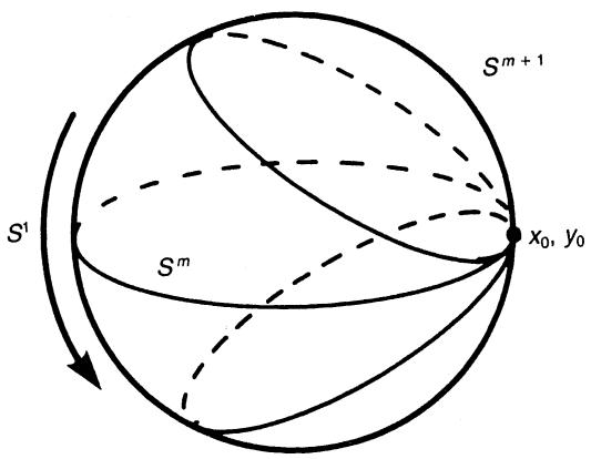
Figure 13.2. The smash product $S^1\wedge S^m\simeq S^{m+1}$ .

$$S^m\wedge S^n=S^{m+n}.\text{\hspace{1em}(13.85)}$$

In the case which interests us, the conditions (13.84) make the direct product $S^1\times S^m$ look topologically like $S^1\wedge S^m=S^{m+1}$ . Thus, $g$ is regarded as a map

from $S^{m+1}$ to $G$ and is classified by ${\pi }_{m+1}(G)$ . Since we have a one-parameter family in the space $\mathfrak{G}={\Omega }^m(G)$ , we also have ${\pi }_{m+1}(G)={\pi }_1(\mathfrak{G})$ . In practice, we take $G=\mathrm{SU}(N)$ for which we have

$${\pi }_{m+1}(\mathrm{SU}(N))=\mathbb{Z}N\ge \frac{1}{2}m+1.\text{\hspace{1em}(13.86)}$$

Now we take a ‘reference’ gauge field $\mathcal{A}$ in the zero instanton sector ${\Omega }_0^m(G)$ for which we may assume, without loss of generality, that the Dirac operator (13.49) has no zero modes. Consider a one-parameter family of gauge potentials

$${\mathcal{A}}^{g(\theta )}(x)\equiv g^{-1}(\theta ,x)(\mathcal{A}(x)+d)g(\theta ,x)\text{\hspace{1em}(13.87)}$$

where $\theta$ parametrizes $S^1$ . In section 13.3, we observed that $|\det \mathrm{i}\hat{D}|$ is gauge invariant (see (13.47)) and only the phase of $\det \mathrm{i}\hat{D}$ may gain an anomalous variation under a gauge transformation. This, in particular, implies that $\det \mathrm{i}\hat{D}$ does not vanish for any $\theta$ . We write

$$\exp \{-W_r[{\mathcal{A}}^{g(\theta )}]\}=\det \mathrm{i}\hat{D}({\mathcal{A}}^{g(\theta )})=[\det \mathrm{i}\bar{\nabla }(\mathcal{A}){]}^{1/2}\exp [\mathrm{i}w(\mathcal{A},\theta )]\text{\hspace{1em}(13.88)}$$

where $\mathrm{i}\overline{\mathcal{V}}$ is the Dirac operator (13.49) and $\exp [\mathrm{i}w(\mathcal{A},\theta )]$ is the anomalous phase associated with the gauge transformation (13.87). Next we consider a two-parameter family of gauge fields ${\mathcal{A}}^{t,\theta }$ $(0\le t\le 1)$ which interpolates between $\mathcal{A}=0$ and ${\mathcal{A}}^{g(\theta )}$ ,

$${\mathcal{A}}^{t,\theta }\equiv t{\mathcal{A}}^{g(\theta )}(0\le t\le 1).\text{\hspace{1em}(13.89)}$$

The parameter space specified by $(t,\theta )$ is considered to be a two-dimensional unit disc $D^2$ with polar coordinates $(t,\theta )$ . On the boundary of the disc, $\partial D^2=S^1$ , the modulus of $\det \mathrm{i}\hat{D}({\mathcal{A}}^{1,\theta })$ is a non-vanishing constant. The phase ${\mathrm{e}}^{\mathrm{i}w(\mathcal{A},\theta )}$ now defines a map $S^1(=\partial D^2)\to S^1(=\mathrm{U}(1))$ ; see figure 13.3. As we move around

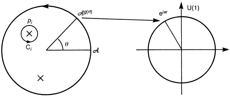
Figure 13.3. The phase of the effective action $W[{\mathcal{A}}^{g(\theta )}]$ defines a map $S^1\to \mathrm{U}(1)$ by $\theta \mapsto {\mathrm{e}}^{\mathrm{i}w(\mathcal{A},\theta )}$ . On the disc, there are points $\{p_i\}$ at which $\det \mathrm{i}\hat{D}({\mathcal{A}}^{t,\theta })$ vanishes. The winding number of the map $S^1\to \mathrm{U}(1)$ is obtained by summing a winding number along $C_i$ .

the boundary of the disc, the phase winds around the unit circle. The winding number of this map is an integer

$$\mathcal{N}=\frac{1}{2\pi }{\int }_0^{2\pi }\frac{\partial w(\mathcal{A},\theta )}{\partial \theta }\mathrm{d}\theta .\text{\hspace{1em}(13.90)}$$

We find below that $\mathcal{N}$ is derived from the Abelian anomaly in $(m+2)$ dimensions.

Exercise 13.2

Show that

$$W[{\mathcal{A}}^{\mathcal{G}(2\pi )}]-W[{\mathcal{A}}^{\mathcal{G}(0)}]=-2\pi \mathrm{i}\mathbb{N}.\text{\hspace{1em}(13.91)}$$

Since $g(2\pi )=g(0)$ , (13.91) may be regarded as a Berry phase.

13.5.1 $m$ dimensions versus $m+2$ dimensions

We recall that our reference gauge field $\mathcal{A}$ supports no zero modes of the operator $\mathrm{i}\hat{D}(\mathcal{A})$ . Since $|\det \mathrm{i}\hat{D}({\mathcal{A}}^{g(\theta )})|=|\det \mathrm{i}\hat{D}(\mathcal{A})|\ne 0$ , the operator $\mathrm{i}\hat{D}({\mathcal{A}}^{g(\theta )})$ does not admit zero modes either. Of course, $\mathrm{i}\hat{D}({\mathcal{A}}^{t,\theta })$ may have zero modes since ${\mathcal{A}}^{t,\theta }$ is not obtained from $\mathcal{A}$ by a gauge transformation in general. Suppose it has a zero mode at $p_i=(t_i,{\theta }_i)$ . We assume they are isolated points. Since $\det \mathrm{i}\hat{D}({\mathcal{A}}^{t,\theta })$ is a regularized product of eigenvalues, it vanishes at $p_i$ . The phase of $\det \mathrm{i}\hat{D}({\mathcal{A}}^{t,\theta })$ may be homotopically non-trivial only around these points. Moreover, the winding number at $p_i$ is determined by the eigenvalue which vanishes at $p_i$ . For example, if ${\lambda }_n(t,\theta )$ vanishes at $p_i$ it should be of the form

$${\lambda }_n(t,\theta )=f(t,\theta ){\mathrm{e}}^{\mathrm{i}{w}_i(t,\theta )}\text{\hspace{1em}(13.92)}$$

where $f(t_i,{\theta }_i)=0$ . The winding number at $p_i$ is

$$m_i=\frac{1}{2\pi }{\int }_{C_i}\frac{\mathrm{d}}{\mathrm{d}s}{w}_i(t,\theta )\mathrm{d}s\text{\hspace{1em}(13.93)}$$

where ${\mathbf{C}}_i$ is a small contour surrounding $p_i$ , see figure 13.3. Continuously deforming the loop $S^1=\partial D^2$ into a sum of small circles ${\mathbf{C}}_i$ enclosing $p_i$ , we find that the total winding number is

$$\mathcal{N}=\frac{1}{2\pi }{\int }_{S^1}\mathrm{d}\theta \frac{\partial }{\partial \theta }w(\mathcal{A},\theta )=\sum m_i.\text{\hspace{1em}(13.94)}$$

Now we show that the winding number $\mathcal{N}$ is related to the index theorem in $(m+2)$ -dimensional space $(m=2l)$ : $\mathcal{N}=\mathrm{ind}\mathrm{i}{\bar{\nabla }}_{m+2}$ where $\mathrm{i}{\bar{\nabla }}_{m+2}$ is the Dirac operator on $S^2\times S^m$ defined later. Let us consider a gauge theory defined on $D^2\times S^m$ whose coordinates are $(t,\theta ,x)$ . To avoid the boundary term, we add another piece, $D^2\times S^m$ , with coordinates $(s,\theta ,x)$ , to form a manifold $S^2\times S^m$ without a boundary; see figure 13.4. We call the patch $(t,\theta )$ the northern hemisphere $U_{\mathrm{N}}$ and $(s,\theta )$ the southern hemisphere $U_{\mathrm{S}}$ . On the equator $S^1$ of $S^2$ , we have $t=s=1$ . We choose the following local gauge potentials

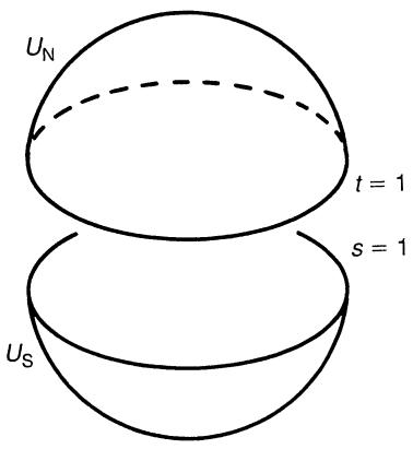
Figure 13.4.

$${\mathcal{A}}_{\mathrm{N}}(t,\theta ,x)={\mathcal{A}}^{t,\theta }+g^{-1}{\mathrm{d}}_{\theta }g(t,\theta )\in U_{\mathrm{N}}\text{\hspace{1em}(13.95a)}$$

$${\mathcal{A}}_{\mathrm{S}}(s,\theta ,x)=\mathcal{A}(s,\theta )\in U_{\mathrm{S}}\text{\hspace{1em}(13.95b)}$$

where $\mathcal{A}$ is the reference gauge field introduced previously. To elevate ${\mathcal{A}}_{\mathrm{N}}={\mathcal{A}}_{\mathrm{N}\mu }\mathrm{d}{x}^{\mu }$ and ${\mathcal{A}}_{\mathrm{S}}={\mathcal{A}}_{\mathrm{S}\mu }\mathrm{d}{x}^{\mu }$ to the globally defined connection on the $G$ bundle over $S^2\times S^m$ we define the $(m+2)$ -dimensional gauge potentials

$${\mathbb{A}}_{\mathrm{N}}(t,\theta ,x)=\left({\mathcal{A}}_t,{\mathcal{A}}_{\theta },{\mathcal{A}}_{\mu }\right)=(0,0,{\mathcal{A}}_{\mathrm{N}\mu })\text{\hspace{1em}(13.96a)}$$

$${\mathbb{A}}_S(s,\theta ,x)=\left({\mathcal{A}}_s,{\mathcal{A}}_{\theta },{\mathcal{A}}_{\mu }\right)=(0,0,{\mathcal{A}}_{S\mu }).\text{\hspace{1em}(13.96b)}$$

On the equator $(t=s=1)$ , we have ${\mathbb{A}}_{\mathrm{N}}=g^{-1}({\mathbb{A}}_{\mathrm{S}}+\Delta )g$ , where $\Delta =\mathrm{d}+{\mathrm{d}}_{\theta }+{\mathrm{d}}_t$ (note that ${\mathrm{d}}_{t}g=0$ ). Thus, $\mathbb{A}=\{{\mathbb{A}}_{\mathrm{N}},{\mathbb{A}}_{\mathrm{S}}\}$ defines a global connection on $S^2\times S^m$ . Consider a Dirac operator $\mathrm{i}{\nabla }_{m+2}$ which couples to $\mathbb{A}$ . The index theorem for $\mathrm{i}{\nabla }_{m+2}$ is given by

$$\mathrm{ind}\mathrm{i}{\bar{\mathcal{V}}}_{m+2}={\mathcal{N}}_{+}-{\mathcal{N}}_{-}={\int }_{S^2\times S^m}{\mathrm{ch}}_{l+1}(\mathbb{F})\text{\hspace{1em}(13.97)}$$

where $\mathbb{F}=\Delta \mathbb{A}+{\mathbb{A}}^2$ and ${\mathcal{N}}_{+}$ $({\mathcal{N}}_{-})$ is the number of $+$ -chirality zero modes of $\mathrm{i}{\overline{\mathcal{V}}}_{m+2}$ (chirality is defined in an $(m+2)$ -space).

Alvarez-Gaume and Ginsparg (1984) have shown, using an adiabatic perturbative computation, that each winding number $m_i$ must be $\pm 1$ . Moreover, the Dirac operator $\mathrm{i}{\nabla }_{m+2}$ has a zero mode at $p_i=(t_i,{\theta }_i)$ with $(m+2)$ -dimensional chirality $\chi =m_i=\pm 1$ . Then the total winding number $\mathcal{N}=\sum m_i$ is given by the index ${\mathcal{N}}_{+}-{\mathcal{N}}_{-}$ . Now we have

$$\mathrm{ind}\mathrm{i}{\nabla }_{m+2}={\int }_{S^2\times S^m}{\mathrm{ch}}_{l+1}(\mathbb{F})=\frac{1}{2\pi }{\int }_0^{2\pi }\mathrm{d}\theta \frac{\partial w(A,\theta )}{\partial \theta }.\text{\hspace{1em}(13.98)}$$

We easily find the non-Abelian anomaly from (13.98) including the normalization. Since ${\mathrm{ch}}_{l+1}(\mathbb{F})=\mathrm{d}{Q}_{m+1}(\mathbb{A},\mathbb{F})$ , we have

$$\begin{array}{rl}{\int }_{S^2\times S^m}{\mathrm{ch}}_{l+1}(\mathbb{F})& ={\int }_{D^2\times S^m}{\mathrm{ch}}_{l+1}\left({\mathbb{F}}_{\mathrm{N}}\right)+{\int }_{D^2\times S^m}{\mathrm{ch}}_{l+1}\left({\mathbb{F}}_{\mathrm{S}}\right)\\ & ={\int }_{S^1\times S^m}{\left[Q_{m+1}\left({\mathbb{A}}_{\mathrm{N}},{\mathbb{F}}_{\mathrm{N}}\right)\right|}_{t=1}-Q_{m+1}\left({\mathbb{A}}_{\mathrm{S}},{\mathbb{F}}_{\mathrm{S}}\right){|}_{s=1}].\end{array}\text{\hspace{1em}(13.99)}$$

From (11.118), we find that

$$\begin{array}{rl}& Q_{m+1}\left({\mathbb{A}}_{\mathrm{N}},{\mathbb{F}}_{\mathrm{N}}\right){|}_{t=1}-Q_{m+1}\left({\mathbb{A}}_{\mathrm{S}},{\mathbb{F}}_{\mathrm{S}}\right){|}_{s=1}\\ & =Q_{m+1}\left(g^{-1}\Delta g,0\right)+\Delta {\alpha }_m\\ & =(-1{)}^l{\left(\frac{\mathrm{i}}{2\pi }\right)}^{l+1}\frac{l!}{(m+1)!}\mathrm{tr}{\left(g^{-1}\Delta g\right)}^{m+1}+\Delta {\alpha }_m.\end{array}\text{\hspace{1em}(13.100)}$$

The index theorem is now given by

$$\mathrm{ind}\mathrm{i}{\nabla }_{m+2}=(-1{)}^l{\left(\frac{\mathrm{i}}{2\pi }\right)}^{l+1}\frac{l!}{(m+1)!}{\int }_{S^1\times S^m}\mathrm{tr}{\left(g^{-1}\Delta g\right)}^{m+1}.\text{\hspace{1em}(13.101)}$$

Theorem 10.7 states that ${\int }_{S^3}\mathrm{tr}(g^{-1}\mathrm{d}g{)}^3$ yields the winding number of the map $g:S^3\to \mathrm{SU}(2)$ . In the same manner, (13.101) represents the winding number of the map $g:S^{m+1}\to G$ and is classified by ${\pi }_{m+1}(G)$ (note that $S^1\wedge S^m=S^{m+1}$ ).

Finally, we show that the non-Abelian anomaly should be identified with $Q_m^1$ . We first note that

$${\int }_{S^1\times S^m}{Q}_{m+1}({\mathbb{A}}_{\mathrm{S}},{\mathbb{F}}_{\mathrm{S}})=0$$

since the integrand is independent of $\mathrm{d}\theta$ and, thus, cannot be a volume element of $S^1\times S^m$ . Then we have

$$\mathrm{ind}\mathrm{i}{\overline{\mathcal{V}}}_{m+2}={\int }_{S^1\times S^m}{Q}_{m+1}\left({\mathcal{A}}^{g(\theta )}+\omega ,{\mathcal{F}}^{g(\theta )}\right)\text{\hspace{1em}(13.102)}$$

where $\omega =g^{-1}{\mathrm{d}}_{\theta }g$ and ${\mathcal{F}}^{g(\theta )}=\mathrm{d}{\mathcal{A}}^{g(\theta )}+({\mathcal{A}}^{g(\theta )}{)}^2=g(\theta {)}^{-1}\mathcal{F}g(\theta )$ . If the integrand in (13.102) is expanded in $\omega$ , only the term linear in $\mathrm{d}\theta$ contributes to the integral. This term $Q_m^1(\omega ,{\mathcal{A}}^{g(\theta )},{\mathcal{F}}^{g(\theta )})$ is proportional to $\mathrm{d}\theta \wedge$ (volume element in $S^m$ ) and, hence, is a volume element of $S^1\times S^m$ . We now have

$$\begin{array}{rl}{\delta }_{\omega }W[\mathcal{A}]& ={\int }_{S^m}\mathrm{tr}\omega {\mathcal{D}}_{\mu }\frac{\delta W[\mathcal{A}]}{\delta {\mathcal{A}}_{\mu }}\\ & ={\mathrm{id}}_{\theta }w(\theta ,\mathcal{A})=2\pi \mathrm{i}{\int }_{S^m}{Q}_m^1(\omega ,{\mathcal{A}}^{g(\theta )},{\mathcal{F}}^{g(\theta )}).\end{array}\text{\hspace{1em}(13.103)}$$

The explicit form of $Q_m^1$ is given by (13.82). For $m=4$ , we find that

$$\begin{array}{rl}\int \mathrm{tr}\omega {\mathcal{D}}_{\mu }\frac{\delta W[\mathcal{A}]}{\delta {\mathcal{A}}_{\mu }}& =2\pi \mathrm{i}{\int }_{S^4}{Q}_4^1(\omega ,{\mathcal{A}}^{g(\theta )},{\mathcal{F}}^{g(\theta )})\\ & =\frac{1}{24{\pi }^2}{\int }_{S^4}\mathrm{tr}\omega \mathrm{d}\left[{\mathcal{A}}^{g(\theta )}\mathrm{d}{\mathcal{A}}^{g(\theta )}+\frac{1}{2}{\left({\mathcal{A}}^{g(\theta )}\right)}^3\right]\end{array}\text{\hspace{1em}(13.104)}$$

Putting $\theta =0$ ( $g=e$ ), we reproduce the anomalous divergence

$${\mathcal{D}}_{\mu }⟨j^{\mu }{⟩}_{\alpha }=\frac{1}{24{\pi }^2}\mathrm{tr}{T}_{\alpha }{ϵ}^{\kappa \lambda \mu \nu }{\partial }_{\kappa }\left[{\mathcal{A}}_{\lambda }{\partial }_{\mu }{\mathcal{A}}_{\nu }+\frac{1}{2}{\mathcal{A}}_{\lambda }{\mathcal{A}}_{\mu }{\mathcal{A}}_{\nu }\right]\text{\hspace{1em}(13.105)}$$

which is in agreement with (13.56). The present method guarantees that the WZ condition yields the correct result. Moreover, it reproduces the anomalous divergence including the normalization which cannot be fixed by the WZ condition alone.

Endnotes

Unplaced source note

The readers may convince themselves by explicitly drawing $S^1\wedge S^1=S^2$ .

来源与版本

正文：英文 · OCR 机器稿 · 待校对

核对状态：OCR 机器稿 · 待校对

原书 PDF

来源版本：second-edition-local

来源 PDF SHA-256：fcd24c3371d092a8c699ccf5cf0765462924b6c48412804231076e8084b1940d

OCR 来源 SHA-256：0b6324f01172a3548cd34382e82fd8bfae574602b6b2cfaa357ba96bc2c35478

OCR 产物 SHA-256：faa5d341dc0844cd43f243dc1c194500cbc8c60f65da2087c900e6f5958a08cf