46.4 Quantization in Coulomb gauge

46.4 Quantization in Coulomb gauge

A diferent method for dealing with the time-independent gauge transformations is to impose an additional gauge condition. For any vector potential satisfying the temporal gauge condition $A_0=0$ , a gauge transformation can be found such that the transformed vector potential satisfies:

Definition (Coulomb gauge)

$A$ vector potential $A_{\mu }$ is said to be in Coulomb gauge if $\nabla \cdot \mathbf{A}=0$

To see that this is possible, note that under a gauge transformation one has

$$\nabla \cdot \mathbf{A}\to \nabla \cdot \mathbf{A}+{\nabla }^2\phi$$

so such a gauge transformation will put a vector potential in Coulomb gauge if we can find a solution to

$${\nabla }^2\phi =-\nabla \cdot \mathbf{A}\text{\hspace{1em}(46.13)}$$

Using Green’s function methods like those of section 12.7, this equation for $\phi$ can be solved, with the result

$$\phi (\mathbf{x})=\frac{1}{4\pi }{\int }_{{\mathbf{R}}^3}\frac{1}{|\mathbf{x}-{\mathbf{x}}^{\prime }|}(\nabla \cdot \mathbf{A}({\mathbf{x}}^{\prime }))d^3{\mathbf{x}}^{\prime }$$

Since in temporal gauge

$$\nabla \cdot \mathbf{E}=-\frac{\partial }{\partial t}\nabla \cdot \mathbf{A}$$

the Coulomb gauge condition automatically implies that Gauss’s law (46.4) will hold. We thus can take as phase space the solutions to the Maxwell equations satisfying the two conditions $A_0=0,\nabla \cdot \mathbf{A}=0$ , with phase space coordinates the pairs $(\mathbf{A}(\mathbf{x}),-\mathbf{E}(\mathbf{x}))$ satisfying the constraints $\nabla \cdot \mathbf{A}=0,\nabla \cdot \mathbf{E}=0$

In Coulomb gauge the one Maxwell equation (46.3) that is not automatically satisfied is, in terms of the vector potential

$$-\frac{{\partial }^2\mathbf{A}}{\partial t^2}=\nabla \times (\nabla \times \mathbf{A})$$

Using the vector calculus identity

$$\nabla \times (\nabla \times \mathbf{A})=\nabla (\nabla \cdot \mathbf{A})-{\nabla }^2\mathbf{A}$$

and the Coulomb gauge condition, this becomes the wave equation

$$\left(\frac{{\partial }^2}{\partial t^2}-{\nabla }^2\right)\mathbf{A}=0\text{\hspace{1em}(46.14)}$$

This is just three copies of the real Klein-Gordon equation for mass $m=0$ although it needs to be supplemented by the Coulomb gauge condition.

One can proceed exactly as for the Klein-Gordon case, using the Fourier transform to identify solutions with functions on momentum space, and quantizing with annihilation and creation operators. The momentum space solutions are given by the Fourier transforms ${\tilde{A}}_j(\mathbf{p})$ and a classical solution can be written in terms of them by a simple generalization of equation 43.8 for the scalar field case

$$A_j(t,\mathbf{x})=\frac{1}{(2\pi {)}^{3/2}}{\int }_{{\mathbf{R}}^3}({\alpha }_j(\mathbf{p})e^{-i{\omega }_{\mathbf{p}}t}{e}^{i\mathbf{p}\cdot \mathbf{x}}+{\overline{\alpha }}_j(\mathbf{p})e^{i{\omega }_{\mathbf{p}}t}{e}^{-i\mathbf{p}\cdot \mathbf{x}})\frac{d^3\mathbf{p}}{\sqrt{2{\omega }_{\mathbf{p}}}}\text{\hspace{1em}(46.15)}$$

where

$${\alpha }_j(\mathbf{p})=\frac{{\tilde{A}}_{j,+}(\mathbf{p})}{\sqrt{2{\omega }_{\mathbf{p}}}},{\overline{\alpha }}_j(\mathbf{p})=\frac{{\tilde{A}}_{j,-}(-\mathbf{p})}{\sqrt{2{\omega }_{\mathbf{p}}}}$$

Here ${\omega }_{\mathbf{p}}=|\mathbf{p}|;$ , and $\begin{array}{r}{\tilde{A}}_{j,+},{\tilde{A}}_{j,}\end{array}$ ₋ are the Fourier transforms of positive and negative energy solutions of 46.14.

The three components ${\alpha }_j(\mathbf{p})$ make up a vector-valued function $\alpha (\mathbf{p})$ . Solutions must satisfy the Coulomb gauge condition $\nabla \cdot \mathbf{A}=0$ , which in momentum space is

$$\mathbf{p}\cdot \mathbf{\alpha }(\mathbf{p})=0\text{\hspace{1em}(46.16)}$$

The space of solutions of this will be two dimensional for each value of $\mathbf{p},$ and we can choose some orthonormal basis

$${ϵ}_1(\mathbf{p}),{ϵ}_2(\mathbf{p})$$

of such solutions (there is a topological obstruction to doing this continuously, but a continuous choice is not necessary). Here the ${ϵ}_{\sigma }(\mathbf{p})\in {\mathbf{R}}^3$ for $\sigma =1$ , 2 are called “polarization vectors”, and satisfy

$$\mathbf{p}\cdot {\mathbf{ϵ}}_1(\mathbf{p})=\mathbf{p}\cdot {\mathbf{ϵ}}_2(\mathbf{p})=0,{\mathbf{ϵ}}_1(\mathbf{p})\cdot {\mathbf{ϵ}}_2(\mathbf{p})=0,|{\mathbf{ϵ}}_1(\mathbf{p}){|}^2=|{\mathbf{ϵ}}_2(\mathbf{p}){|}^2=1$$

They provide an orthonormal basis of the tangent space at p to the sphere of radius |p|.

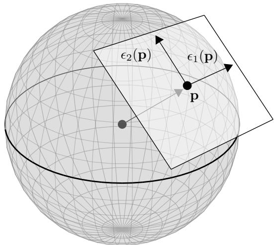
Figure 46.1: Polarization vectors at a point $p$ in momentum space.

The space of solutions is thus two copies of the space of solutions of the massless Klein-Gordon case. The quantum field for the theory of photons is then

$$\begin{array}{rlr}& & \hat{\mathbf{A}}(t,\mathbf{x})=\frac{1}{(2\pi {)}^{3/2}}{\int }_{{\mathbf{R}}^3}{\sum }_{\sigma =1,2}({ϵ}_{\sigma }(\mathbf{p})a_{\sigma }(\mathbf{p})e^{-i{\omega }_{\mathbf{p}}t}{e}^{i\mathbf{p}\cdot \mathbf{x}}\\ & & +{ϵ}_{\sigma }(\mathbf{p})a_{\sigma }^{†}(\mathbf{p})e^{i{\omega }_{\mathbf{p}}t}{e}^{-i\mathbf{p}\cdot \mathbf{x}})\frac{d^3\mathbf{p}}{\sqrt{2{\omega }_{\mathbf{p}}}}\end{array}\text{\hspace{1em}(46.17)}$$

where $a_{\sigma },a_{\sigma }^{†}$ are annihilation and creation operators satisfying

$$[a_{\sigma }(\mathbf{p}),a_{{\sigma }^{\prime }}^{†}({\mathbf{p}}^{\prime })]={\delta }_{\sigma {\sigma }^{\prime }}{\delta }^3(\mathbf{p}-{\mathbf{p}}^{\prime })$$

The state space of the theory will describe an arbitrary number of particles for each value of the momentum p (called photons), obeying the energy-momentum relation ${\omega }_{\mathbf{p}}=|\mathbf{p}|$ , with a two dimensional degree of freedom describing their polarization.

Note the appearance here of the following problem: unlike the scalar field case (equation 43.8) where the Fourier coeficients were unconstrained functions, here they satisfy a condition (equation 46.16), and the ${\alpha }_j(\mathbf{p})$ cannot simply be quantized as independent annihilation operators for each $j.$ Solving equation 46.16 and reducing the number of degrees of freedom by introducing the polarization vectors ${ϵ}_{\sigma }$ involves an arbitrary choice and makes the properties of the theory under the action of the Lorentz group much harder to understand. A similar problem for solutions to the Dirac equation will appear in chapter 47.

Previous section: 46.3 Gauss’s law and time-independent gauge transformations · Next section: 46.5 Space-time symmetries · 中文版本

来源与版本

正文：英文 · OCR 机器稿 · 待校对

核对状态：OCR 机器稿 · 待校对

原书 PDF · 印刷页 494、495、496、497、498、499、500、501、502、503、504、505、506、507、508、509、510

来源版本：2025-10-20

来源 PDF SHA-256：5a1941b2443b54d5db3d055f1e5ba390429b7a728475258017aaac87ee85a837

OCR 来源 SHA-256：490bb084314aadb3aedb08406a9dba1bd18c81c7b4d048ac90fd182ad89cc52b

OCR 产物 SHA-256：490bb084314aadb3aedb08406a9dba1bd18c81c7b4d048ac90fd182ad89cc52b