1.3 A First Look at the Schwarzschild Metric

Physics was born from our attempts to understand the motion of the planets. The problem was largely solved by Newton, who was able to derive Kepler’s laws of planetary motion from the gravitational force law. This was described in some detail in our first lecture course on Dynamics and Relativity.

Newton’s laws are not the end of the story. There are relativistic corrections to the orbits of the planets that can be understood by computing the geodesics in the background of a star.

To do this, we first need to understand the metric created by a star. This will be derived in Section 6. For now, we simply state the result: a star of mass M gives rise to a curved spacetime given by

$$d{s}^2=-\left(1-\frac{2GM}{r{c}^2}\right)d{t}^2+{\left(1-\frac{2GM}{r{c}^2}\right)}^{-1}d{r}^2+r^2(d{\theta }^2+{\sin }^2\theta d{\varphi }^2)$$

This is the Schwarzschild metric. The coordinates $\theta$ and $\varphi$ are the usual spherical polar coordinates, with $\theta \in [0,\pi ]$ and $\varphi \in [0,2\pi )$

We will have to be patient to fully understand all the lessons hiding within this metric. But we can already perform a few sanity checks. First, note that far from the star, as $r\to \infty$ , it coincides with the Minkowski metric as it should. Secondly, the $g_{00}$ component is given by

$$g_{00}=-\left(1+\frac{2\Phi }{c^2}\right)\text{ with }\Phi (r)=-\frac{GM}{r}$$

which agrees with our expectation (1.24) with $\Phi =-GM/r$ the usual Newtonian potential for an object of mass $M$

The Schwarzschild metric also has some strange things going on. In particular, the $g_{rr}$ component diverges at $r=R_s$ where

$$R_s=\frac{2GM}{c^2}$$

is called the Schwarzschild radius. This is the event horizon of a black hole and will be explored more fully in Section 6. However, it turns out that space around any spherically symmetric object, such as a star, is described by the Schwarzschild metric, now restricted to $r>R_{\mathrm{star}}$ , with $R_{\mathrm{star}}$ the radius of the star.

In what follows we will mostly view the Schwarzschild metric as describing the spacetime outside a star, and treat the planets as test particles moving along geodesics in this metric. We will also encounter a number of phenomena that happen close to $r=R_s;$ these are relevant only for black holes, since $R_{\mathrm{star}}\gg R_s$ . However we will, for now, avoid any discussion of what happens if you venture past the event horizon.

1.3.1 The Geodesic Equations

Our first task is to derive the equations for a geodesic in the Schwarzschild background. To do this, we use the quick and easy method of looking at the action (1.32) for a particle moving in the Schwarzschild spacetime,

$$\begin{array}{rl}& S_{\mathrm{useful}}=\int d\tau L=\int d\tau g_{\mu \nu }(x){\dot{x}}^{\mu }{\dot{x}}^{\nu }\\ & =\int d\tau \left[-A(r)c^2{\dot{t}}^2+A^{-1}(r){\dot{r}}^2+r^2({\dot{\theta }}^2+{\sin }^2\theta {\dot{\varphi }}^2)\right]\end{array}\text{\hspace{1em}(1.35)}$$

with $A(r)=1-R_s/r$ and ${\dot{x}}^{\mu }=d{x}^{\mu }/d\tau$

When we solved the Kepler problem in Newtonian mechanics, we started by using the conservation of angular momentum to restrict the problem to a plane. We can use the same trick here. We first look at the equation of motion for ${\theta }_{;}$

$$\frac{d}{d\tau }\left(\frac{dL}{d\dot{\theta }}\right)-\frac{dL}{d\theta }=0\Rightarrow \frac{d}{d\tau }(r^2\dot{\theta })=r^2\sin \theta \cos \theta {\dot{\varphi }}^2$$

This tells us that if we kick the particle of in the $\theta =\pi /2$ plane, with $\dot{\theta }=0$ , then it will remain there for all time. This is the choice we make.

We still have to compute the magnitude of the angular momentum. Like many conserved quantities, this follows naturally by identifying the appropriate ignorable coordinate. Recall that if the Lagrangian is independent of some specific coordinate x then the Euler-Lagrange equations immediately give us a conserved quantity,

$$\frac{dL}{dx}=0\Rightarrow \frac{d}{d\tau }\left(\frac{dL}{d\dot{x}}\right)=0$$

This is a baby version of Noether’s theorem.

The action (1.35) has two such ignorable coordinates, t and $\varphi .$ . The conserved quantity associated to ϕ is the magnitude of the angular momentum, l. (Strictly, the angular momentum per unit mass.) Restricting to the $\theta =\pi /2$ plane, we define this to be

$$2l=\frac{dL}{d\dot{\varphi }}=2r^2\dot{\varphi }\text{\hspace{1em}(1.36)}$$

where the factor of 2 on the left-hand side arises because the kinetic terms in (1.35) don’t come with the usual factor of $1/2$ . Meanwhile, the conserved quantity associated to $t(\tau )$ is

$$-2E=\frac{dL}{d\dot{t}}=-2A(r)c^2\dot{t}\text{\hspace{1em}(1.37)}$$

The label $E$ is not coincidence: it should be interpreted as the energy of the particle (or, strictly, the energy divided by the rest mass). To see this, we look far away: as $r\to \infty$ we have $A(r)\approx 1$ and we return to Minkowski space. Here, we know from our lectures on Special Relativity that $dt/d\tau =\gamma$ . We then have $E\to \gamma c^2$ as $r\to \infty$ . But this is precisely the energy per unit rest mass of a particle in special relativity.

We should add to these conservation laws the constraint (1.33) which tells us that the geodesic is parameterised by proper time. Restricting to $\theta =\pi /2$ and $\dot{\theta }=0$ , this becomes

$$-A(r)c^2{\dot{t}}^2+A^{-1}(r){\dot{r}}^2+r^2{\dot{\varphi }}^2=-c^2\text{\hspace{1em}(1.38)}$$

If we now substitute in the expressions for the conserved quantities l and E, this constraint can be rewritten as

$$\frac{1}{2}{\dot{r}}^2+V_{\mathrm{eff}}(r)=\frac{1}{2}\frac{E^2}{c^2}\text{\hspace{1em}(1.39)}$$

The effective potential $V_{\mathrm{eff}}(r)$ includes the factor $A(r)$ which we now write out in full,

$$V_{\mathrm{eff}}(r)=\frac{1}{2}\left(c^2+\frac{l^2}{r^2}\right)\left(1-\frac{2GM}{r{c}^2}\right)\text{\hspace{1em}(1.40)}$$

Our goal is to solve for the radial motion (1.39). We subsequently use the expression (1.36) to solve for the angular motion and, in this way, determine the orbit.

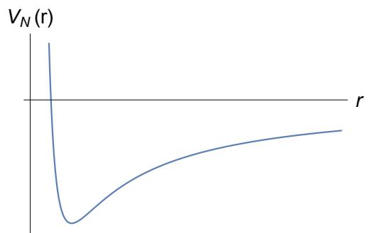
Figure 3. The effective potential for Newtonian gravity.

1.3.2 Planetary Orbits in Newtonian Mechanics

Before we solve the full geodesic equations, it is useful to first understand how they differ from the equations of Newtonian gravity. To see this, we write

$$V_{\mathrm{eff}}(r)=\frac{c^2}{2}-\frac{GM}{r}+\frac{l^2}{2r^2}-\frac{l^{2}GM}{r^3{c}^2}$$

The non-relativistic limit is, roughly, $c^2\to \infty$ . This means that we drop the final term in the potential that scales as $1/r^3$ . (Since c is dimensionful, it is more accurate to say that we restrict to situations with $l^{2}GM/r^3\ll c^2.)$ Meanwhile, we expand the relativistic energy per unit mass in powers of $1/c^2$ 2

$$E=c^2+E_N+\dots$$

where $E_N$ is the non-relativistic energy and … are terms suppressed by $1/c^2$ . Substituting these expressions into (1.39), we find

$$\frac{1}{2}{\dot{r}}^2+V_N(r)=E_N$$

where $V_N$ is the non-relativistic potential which includes both the Newtonian gravitational potential and the angular momentum barrier,

$$V_N(r)=-\frac{GM}{r}+\frac{l^2}{2r^2}$$

These are precisely the equations that we solved in our first course on classical mechanics. (See Section 4.3 of the lectures on Dynamics and Relativity.) The only difference is that $r(\tau )$ is parameterised by proper time τ rather than the observers time t. However, these coincide in the non-relativistic limit that we care about.

We can build a lot of intuition for the orbits by looking at the potential $V_N(r)$ as shown in Figure 3. At large distances, the attractive $-1/r$ gravitational potential dominates, while the angular momentum prohibits the particles from getting too close to the origin, as seen in the $+1/r^2$ term which dominates at short distances. The potential has a minimum at

$$V^{\prime }(r_{\star })=\frac{GM}{r_{\star }^2}-\frac{l^2}{r_{\star }^3}=0\Rightarrow r_{\star }=\frac{l^2}{GM}$$

A particle can happily sit at $r=r_{\star }$ for all time. This circular orbit always has energy $E_N<0$ , reflecting the fact that $V_N(r_{\star })<0$

Alternatively, the particle could oscillate back and forth about the minima. This happens provided that $E_N<0$ so that the particle is unable to escape to $r\to \infty$ . This motion describes an orbit in which the distance to the origin varies; we’ll see below that the shape of the orbit is an ellipse. Finally, trajectories with $E_N\ge 0$ describe fly-bys, in which the particle approaches the star, but gets only so close before flying away never to be seen again.

The discussion above only tells us about the radial motion. To determine the full orbit, we need to use the angular momentum equation $\dot{\varphi }=l/r^2$ . Let’s remind ourselves how we solve these coupled equations. We start by employing a standard trick of working with the new coordinate

$$u=\frac{1}{r}$$

We then view this inverse radial coordinate as a function of the angular variable: $u=$ $u(\varphi )$ . This works out nicely, since we have

$$\dot{u}=\frac{du}{d\varphi }\dot{\varphi }=l{u}^2\frac{du}{d\varphi }$$

where in the last equality, we’ve used angular momentum conservation (1.36) to write $\dot{\varphi }=l{u}^2$ . Using this, we have

$$\dot{r}=-\frac{1}{u^2}\dot{u}=-l\frac{du}{d\varphi }\text{\hspace{1em}(1.41)}$$

The equation giving conservation of energy is then

$${\left(\frac{du}{d\varphi }\right)}^2+{\left(u-\frac{GM}{l^2}\right)}^2=\frac{2E_N}{l^2}+\frac{G^2{M}^2}{l^4}\text{\hspace{1em}(1.42)}$$

But this is now straightforward to solve. We choose to write the solution as

$$u(\varphi )=\frac{GM}{l^2}(1+e\cos \varphi )\text{\hspace{1em}(1.43)}$$

Back in our original radial variable, we have

$$r(\varphi )=\frac{l^2}{GM}\frac{1}{1+e\cos \varphi }\text{\hspace{1em}(1.44)}$$

This is the equation for a conic section, with the eccentricity given by

$$e=\sqrt{1+\frac{2E_N{l}^2}{G^2{M}^2}}$$

The shape of the orbit depends on e. A particle with $E_N\ge 0$ is not in a bound orbit, and traces out a hyperbola for $e>1$ and a parabola for $e=1$ . Planets, in contrast, have energy $E_N<0$ and, correspondingly, eccentricity $e<1$ . In this case, the orbits are ellipses.

To compare with the relativistic result later, we note an important feature of the Newtonian orbit: it does not precess. To see this, note that for our solution (1.44) the point at which the planet is closest to the origin – known as the perihelion – always occurs at the same point $\varphi =0$ in the orbit.

1.3.3 Planetary Orbits in General Relativity

We now repeat this analysis for the full relativistic motion of a massive particle moving along a geodesic in the Schwarzschild metric. We have seen that the effective potential takes the form (1.40)

$$V_{\mathrm{eff}}(r)=\frac{c^2}{2}-\frac{GM}{r}+\frac{l^2}{2r^2}-\frac{GM{l}^2}{r^3{c}^2}$$

The relativistic correction scales as $-1/r^3$ and changes the Newtonian story at short distances, since it ensures that the potential $V_{\mathrm{eff}}(r)\to -\infty$ as $r\to 0$ . Indeed, the potential always vanishes at the Schwarzschild radius $r=R_s=2GM/c^2$ , with $V_{\mathrm{eff}}(R_s)=0$

The potential takes different shapes, depending on the size of the angular momentum. To see this, we compute the critical points

$$V_{\mathrm{eff}}^{\prime }(r)=\frac{GM}{r^2}-\frac{l^2}{r^3}+\frac{3GM{l}^2}{r^4{c}^2}=0\Rightarrow GM{r}^2-l^{2}r+\frac{3GM{l}^2}{c^2}=0\text{\hspace{1em}(1.45)}$$

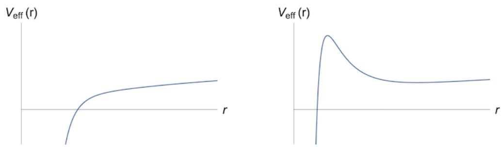
Figure 4. On the left: the effective potential for a massive particle when $l^2{c}^2<12G^2{M}^2$ On the right: when $l^2{c}^2>12G^2{M}^2$

If the discriminant is positive, then this quadratic equation has two solutions. This occurs when the angular momentum is suitably large.

$$l^2>\frac{12G^2{M}^2}{c^2}$$

In this case, the potential looks like the figure shown on the right. We call the two solutions to the quadratic equation (1.45), $r_{+}$ and $r_{-}$ with $r_{+}>r_{-}$ . The outermost solution $r_{+}$ is a minimum of the potential and corresponds to a stable circular orbit; the innermost solution $r_{-}$ is a maximum of the potential and corresponds to an unstable circular orbit.

As in the Newtonian setting, there are also non-circular orbits in which the particle oscillates around the minimum. However, there is no reason to think these will, in general, remain elliptical. We will study some of their properties below.

Note also that, in contrast to the Newtonian case, the angular momentum barrier is now finite: no matter how large the angular momentum, a particle with enough energy (in the form of ingoing radial velocity) will always be able to cross the barrier, at which point it plummets towards $r=0$ . We will say more about this in Section 6 when we discuss black holes.

If the angular momentum is not large enough,

$$l^2<\frac{12G^2{M}^2}{c^2}$$

then the potential $V_{\mathrm{eff}}(r)$ has no turning points and looks like the right-hand figure. In this case, there are no stable orbits; all particles will ultimately fall towards the origin.

The borderline case is $l^2=12G^2{M}^2/c^2$ . In this case the turning point is a saddle at

$$r_{\mathrm{ISCO}}=\frac{6GM}{c^2}\text{\hspace{1em}(1.46)}$$

This is the innermost stable circular orbit. There can be no circular orbits at distances $r<r_{\mathrm{ISCO}}$ , although it is possible for the non-circular orbits to extend into distances $r<r_{\mathrm{ISCO}}$

The innermost stable orbit plays an important role in black hole astrophysics, where it marks the inner edge of the accretion disc which surrounds the black hole. Roughly speaking, this is seen in the famous photograph captured by the Event Horizon Telescope. Here, the “roughly speaking” is partly because the light really emerges from the socalled photon sphere, which is similar to the

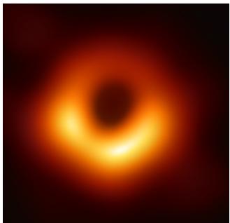
ISCO, but for light, and partly because the light emitted from the accretion disc is warped in a dramatic fashion, so what we see is very different from what is there! (Furthermore, the black hole in the picture almost certainly rotating. This makes r_ISCO smaller than $6GM/c^2$ and the picture significantly harder to interpret.)

We could also ask: how close can a non-circular orbit get? This occurs in the limit $l\to \infty$ , where a quick calculation shows that the maximum of $V_{\mathrm{eff}}$ tends to $r_{-}\to 3GM/c^2$ . This is the closest that any timelike geodesic can get if it wishes to return.

Perihelion Precession

To understand the orbits in more detail, we can attempt to solve the equations of motion. We follow our Newtonian analysis, introducing the inverse parameter $u=1/r$ and converting $\dot{r}$ into $du/d\varphi$ . Our equation (1.39) becomes

$${\left(\frac{du}{d\varphi }\right)}^2+u^2-\frac{2GM}{l^2}u-\frac{2GM}{c^2}{u}^3=\frac{E^2}{l^2{c}^2}-\frac{c^2}{l^2}$$

This equation is considerably harder than our Newtonian orbit equation (1.42). To proceed, it’s simplest to first differentiate again with respect to $\varphi .$ This gives

$$\frac{d^{2}u}{d{\varphi }^2}+u-\frac{GM}{l^2}-\frac{3GM}{c^2}{u}^2=0$$

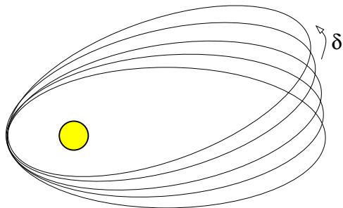
Figure 5. The precession of the perihelion (or aphelion) of an almost elliptical orbit.

where we have assumed that $du/d\varphi \ne 0$ , which means that we are neglecting the simple circular solution. The equation above differs from the analogous Newtonian equation by the final term (which indeed vanishes if we take $c^2\to \infty )$ . There is no closed-form solution to this equation, but we can make progress by working perturbatively. To this end, we define the dimensionless parameter

$$\beta =\frac{3G^2{M}^2}{l^2{c}^2}$$

and write the orbit equation as

$$\frac{d^{2}u}{d{\varphi }^2}+u-\frac{GM}{l^2}=\beta \frac{l^2{u}^2}{GM}\text{\hspace{1em}(1.47)}$$

We will assume $\beta \ll 1$ and look for series solutions of the form

$$u=u_0+\beta u_1+{\beta }^2{u}_2+\dots$$

To leading order, we can ignore the terms proportional to $\beta$ on the right-hand-side of (1.47). This gives us an equation for $u_0$ which is identical to the Newtonian orbit

$$\frac{d^2{u}_0}{d{\varphi }^2}+u_0-\frac{GM}{l^2}=0\Rightarrow u_0(\varphi )=\frac{GM}{l^2}(1+e\cos \varphi )$$

We now feed this back into the equation (1.47) to get an equation for $u_1$ ,

$$\frac{d^2{u}_1}{d{\varphi }^2}+u_1=\frac{l^2}{GM}{u}_0^2=\frac{GM}{l^2}\left[\left(1+\frac{e^2}{2}\right)+2e\cos \varphi +\frac{e^2}{2}\cos 2\varphi \right]$$

You can check that this is solved by

$$u_1=\frac{GM}{l^2}\left[\left(1+\frac{e^2}{2}\right)+e\varphi \sin \varphi -\frac{e^2}{6}\cos 2\varphi \right]$$

We could proceed to next order in ${\beta }_{\pm }$ , but the first correction $u_1$ will be sufficient for our purposes.

The interesting term is the ϕ sin ϕ in $u_1$ . This is not periodic in $\varphi$ and it means that the orbit no longer closes: it sits at a different radial value at $\varphi =0$ and $\varphi =2\pi$ . To illustrate this, we ask: when is the particle closest to origin? This is the perihelion of the orbit. It occurs when

$$\frac{du}{d\varphi }\approx \frac{d(u_0+\beta u_1)}{d\varphi }=0\Rightarrow -e\sin \varphi +\beta \left(e\sin \varphi +e\varphi \cos \varphi +\frac{e^2}{3}\sin 2\varphi \right)=0$$

Clearly this is solved by $\varphi =0$ . The next solution is at $\varphi =2\pi +\delta$ where, due to our perturbative expansion, δ will be small. Expanding our expression above, and dropping terms of order ${\delta }^2$ and $\beta \delta$ , we find the precession of the perihelion given by

$$\delta =2\pi \beta =6\pi \frac{G^2{M}^2}{l^2{c}^2}\text{\hspace{1em}(1.48)}$$

For planets orbiting the Sun, the perihelion shift depends only on the angular momentum l of the planet and the mass of the Sun, denoted $M_{\odot }$ . The latter is $M_{\odot }\approx$ $2\times 10^{30}$ kg, corresponding to the length scale

$$\frac{G{M}_{\odot }}{c^2}\approx 1.5\times 10^3\mathrm{m}$$

If a planet on an almost-circular orbit of radius $r$ orbits the sun in a time $T,$ then the angular momentum (1.36) is

$$l=\frac{2\pi r^2}{T}$$

Recall that Kepler’s third law (which follows from the inverse square law) tells us that $T\propto r^{3/2}$ . This means that $l\propto r^{1/2}$ and, correspondingly, the perihelion shift (1.48) is proportional to $\delta \propto 1/r$ . We learn that the effect should be more pronounced for planets closest to the Sun.

The closest planet to the Sun is Mercury which, happily, is also the only planet whose orbit differs significantly from a circle; it has eccentricity $e\approx 0.2$ , the radius varying from 4.6 to $7\times 10^{10}$ m. Mercury orbits the Sun once every 88 days but, in fact, we don’t need to use this to compute the angular momentum and precession. Instead, we can invoke the elliptic formula (1.44) which tells us that the minimum $r_{-}$ and maximum distance $r_{+}$ is given by

$$r_{\pm }=\frac{l^2}{GM}\frac{1}{1\mp e}\Rightarrow l^2=GM{r}_{+}(1-e)\text{\hspace{1em}(1.49)}$$

from which we get the precession

$$\delta =\frac{6\pi GM}{c^2}\frac{1}{r_{+}(1-e)}$$

Plugging in the numbers gives $\delta \approx 5.0\times 10^{-7}$ . This is rather small. However, the perihelion precession is cumulative. Over a century, Mercury completes 415 orbits, giving the precession of $2.1\times 10^{-4}$ per century.

The result above is quoted in radians. Astronomers prefer units of arcseconds, with 3600 arcseconds (denoted as $3600^{\prime \prime })$ in a degree and, of course, 360 degrees in $2\pi$ radians. This means that $1^{\prime \prime }\approx 4.8\times 10^{-6}$ radians. Our calculation from general relativity gives $43^{\prime \prime }$ per century as the shift in the perihelion. This was one of the first successful predictions of the theory. Subsequently, the perihelion shift of Venus and Earth has been measured and is in agreement with the predictions of general relativity.

1.3.4 The Pull of Other Planets

The general relativistic contribution of $43^{\prime \prime }$ per century is not the full story. In fact the observed perihelion shift of Mercury is much larger, at around $575^{\prime \prime }$ . The vast majority of this is due to the gravitational force of other planets and can be understood entirely within the framework of Newtonian gravity. For completeness, we now give an estimate of these effects.

We start by considering the effect of single, heavy planet with mass $M^{\prime }$ , orbiting at a distance R from the Sun. Of course, the 3-body problem in Newtonian gravity is famously hard. However, there is an approximation which simplifies the problem tremendously: we consider the outer planet to be a circular ring, with mass per unit length given by $M^{\prime }/2\pi R$

It’s not obvious that this is a good approximation. Each of the outer planets takes significantly longer to orbit the Sun than Mercury. This suggests for any given orbit of Mercury, it would be more appropriate to treat the position of the outer planets to be fixed. (For example, it takes Jupiter 12 years to orbit the Sun, during which time Mercury has completed 50 orbits.) This means that the perihelion shift of Mercury depends on the position of these outer planets and that’s a complicated detail that we’re happy to ignore. Instead, we want only to compute the total perihelion shift of Mercury averaged over a century. And for this, we may hope that the ring approximation, in which we average over the orbit of the outer planet first, suffices.

In fact, as we will see, the ring approximation is not particularly good: the calculation is non-linear and averaging over the position of the outer planet first does not commute with averaging over the orbits of Mercury. This means that we will get a ballpark figure for the perihelion precession of Mercury but, sadly, not one that is accurate enough to test relativity.

We would like to determine the Newtonian potential felt by a planet which orbits a star of mass M and is surrounded, in the same plane, by a ring of density $M^{\prime }/2\pi R$ . The geometry is shown in the figure. Obviously, the potential (per unit mass) from the star is

$$V_{\mathrm{star}}(r)=-\frac{GM}{r}$$

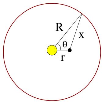
We need to calculate the potential (per unit mass) from the ring. This is

$$V_{\mathrm{ring}}(r)=-\frac{G{M}^{\prime }}{2\pi }{\int }_0^{2\pi }d\theta \frac{1}{x(\theta )}\mathrm{with}{x}^2=R^2+r^2-2Rr\cos \theta \text{\hspace{1em}(1.50)}$$

We use the fact that Mercury is much closer to the Sun than the other planets and Taylor expand the integral in $r^2/R^2$ . To leading order we have

$$V_{\mathrm{ring}}(r)=-\frac{G{M}^{\prime }}{R}\left[1+\frac{1}{4}{\left(\frac{r}{R}\right)}^2+\dots \right]$$

Dropping constant terms, we learn that the effective potential (per unit mass) experienced by Mercury is, to leading order,

$$V_{\mathrm{eff}}(r)=-\frac{GM}{r}+\frac{l^2}{2r^2}-\sum _i\frac{G{M}_i^{\prime }}{4}\frac{r^2}{R_i^3}+\dots$$

where we’ve included the angular momentum barrier and the sum is over all the outer planets. In what follows, we must assume that the $r^2$ correction term is suitably small so that it doesn’t destabilise the existence of orbits. Obviously, this is indeed the case for Mercury.

Now we can follow our calculation for the perihelion precession in general relativity. Conservation of energy tells us

$$\frac{1}{2}{\dot{r}}^2+V_{\mathrm{eff}}(r)=E$$

Working with everyone’s favourite orbit variable, $u=1/r$ , viewed as $u=u(\varphi )$ , the general relativistic equation (1.47) is replaced by

$$\frac{d^{2}u}{d{\varphi }^2}+u-\frac{GM}{l^2}=-\alpha \frac{(GM{)}^4}{l^8{u}^3}\text{\hspace{1em}(1.51)}$$

where this time our small dimensionless parameter is

$$\alpha =\frac{l^6}{2G^3{M}^4}\sum _i\frac{M_i^{\prime }}{R_i^3}=\frac{(1-e{)}^3}{2}\sum _i\frac{M_i^{\prime }}{M}{\left(\frac{r_{+}}{R_i}\right)}^3$$

where, in the second equality, we’ve used (1.49); here M is the mass of the Sun, $r_{+}$ is the outermost radius of Mercury’s orbit, and $e\approx 0.2$ is the eccentricity of Mercury’s orbit. We safely have $\alpha \ll 1$ and so we look for series solutions of the form

$$u=u_0+\alpha u_1+{\alpha }^2{u}_2+\dots$$

We’ve already met the leading order solution, $u_0(\varphi )=(GM/l^2)(1+e\cos \varphi )$ with $e$ the eccentricity of the planet’s orbit. Feeding this into (1.51), we get an equation for the first correction

$$\frac{d^2{u}_1}{d{\varphi }^2}+u_1=-\frac{(GM{)}^4}{l^8}\frac{1}{u_0^3}=-\frac{GM}{l^2}\frac{1}{(1+e\cos \varphi {)}^3}$$

This equation is somewhat harder to solve than the general relativistic counterpart. To proceed, we will assume that the eccentricity is small, $e\ll 1$ , and solve the equation to leading order in $e.$ Then this equation becomes

$$\frac{d^2{u}_1}{d{\varphi }^2}+u_1=-\frac{GM}{l^2}(1-3e\cos \varphi )$$

which has the solution

$$u_1=\frac{GM}{l^2}\left(-1+\frac{3e}{2}\varphi \sin \varphi \right)$$

The precession of the perihelion occurs when

$$\frac{du}{d\varphi }=0\Rightarrow -e\sin \varphi +\frac{3e\alpha }{2}(\sin \varphi +\varphi \cos \varphi )=0$$

As in the relativistic computation, this is solved by $\varphi =0$ and by $\varphi =2\pi +\delta$ where, to leading order, the shift of the perihelion is given by

$$\delta =3\pi \alpha =\frac{3\pi }{2}\sum _i\frac{M_i^{\prime }}{M}{\left(\frac{r_0}{R_i}\right)}^3$$

with $r_0=(1-e)r_{+}$ . Once again, we can put the numbers in. The mass of the Sun is $M=M_{\odot }\approx 2\times 10^{30}$ kg. The formula is very sensitive to the radius of Mercury’s orbit: we use $r_0\approx 5.64\times 10^{10}$ m. The relevant data for the other planets is then

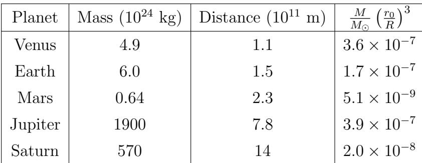
A quick glance at this table shows that the largest contributions come from Jupiter (because of its mass) and Venus (because of it proximity), with the Earth in third place. (The contributions from Uranus, Neptune and Pluto are negligible.)

Adding these contributions, we find $\delta \approx 40\times 10^{-7}$ radians per orbit. This corresponds to $344^{\prime \prime }$ per century, significantly larger than the $43^{\prime \prime }$ per century arising from general relativity but not close to the correct Newtonian value of $532^{\prime \prime }$

Higher Order Contributions

Our analysis above gave us a result of $380^{\prime \prime }$ per century for the perihelion shift of Mercury. A more precise analysis gives $532^{\prime \prime }$ coming from the Newtonian pull of the other planets.

We made a number of different approximations in the discussion above. But the one that introduced the biggest error turns out to be truncating the ring potential (1.50) at leading order in $r/R$ . This, it turns out, is particularly bad for Venus since its orbit compared to Mercury is only $(r_0/R)\approx 0.5$ . To do better, we can expand the potential (1.50) to higher orders. We have

$$\begin{array}{rl}& V_{\mathrm{ring}}(r)=-\frac{G{M}^{\prime }}{2\pi R}{\int }_0^{2\pi }d\theta \frac{1}{\sqrt{R^2+r^2-2Rr\cos \theta }}\\ & =-\frac{G{M}^{\prime }}{R}\left[1+\frac{1}{4}{\left(\frac{r}{R}\right)}^2+\frac{9}{64}{\left(\frac{r}{R}\right)}^4+\frac{25}{256}{\left(\frac{r}{R}\right)}^6+\dots \right]\end{array}$$

An identical calculation to the one above now gives a corresponding perturbative expansion for the perihelion shift,

$$\delta =\pi \sum _i\frac{M_i^{\prime }}{M}\left[\frac{3}{2}{\left(\frac{r_0}{R_i}\right)}^3+\frac{45}{16}{\left(\frac{r_0}{R_i}\right)}^5+\frac{525}{128}{\left(\frac{r_0}{R_i}\right)}^7+\dots \right]$$

with $r_0=(1-e)r_{+}$ the mean orbit of Mercury. The extra terms give significant contributions for Venus, and smaller for Earth. Using the value of $r_0\approx 5.64\times 10^{10}$ m and the slightly more accurate $R^{\prime }\approx 10.6\times 10^{10}$ m for Venus, the sum of the contributions gives $\delta \approx 59\times 10^{-7}$ radians per orbit, or $507^{\prime \prime }$ per century, somewhat closer to the recognised value of $532^{\prime \prime }$ per century but still rather short.

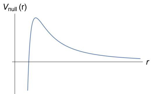
Figure 6. The effective potential for null geodesics in the Schwarzschild metric.

1.3.5 Light Bending

It is straightforward to extend the results above to determine the null geodesics in the Schwarzschild metric. We continue to use the equations of motion derived from $S_{\mathrm{useful}}$ in (1.35). But this time we replace the constraint (1.38) with the null version (1.34), which reads

$$-A(r)c^2{\dot{t}}^2+A^{-1}(r){\dot{r}}^2+r^2{\dot{\varphi }}^2=0$$

The upshot is that we can again reduce the problem to radial motion,

$$\frac{1}{2}{\dot{r}}^2+V_{\mathrm{null}}(r)=\frac{1}{2}\frac{E^2}{c^2}\text{\hspace{1em}(1.52)}$$

but now with the effective potential (1.40) replaced by

$$V_{\mathrm{null}}(r)=\frac{l^2}{2r^2}\left(1-\frac{2GM}{r{c}^2}\right)$$

A typical potential is shown in Figure 6. Note that, as $r\to \infty$ , the potential asymptotes to zero from above, while $V_{\mathrm{null}}\to -\infty \mathrm{as}r\to 0$ . The potential has a single maximum at

$$V_{\mathrm{null}}^{\prime }(r_{\star })=-\frac{l^2}{r_{\star }^3}+\frac{3GM{l}^2}{r_{\star }^4{c}^2}=0\Rightarrow r_{\star }=\frac{3GM}{c^2}\text{\hspace{1em}(1.53)}$$

We learn that there is a distance, $r_{\star }$ , at which light can orbit a black hole. This is known as the photon sphere. The fact that this sits on a maximum of the potential means that this orbit is unstable. In principle, focussing effects mean that much of the light emitted from an accretion disc around a non-rotating black hole emerges from the photon sphere. In practice, it seems likely that photograph of the Event Horizon Telescope does not have the resolution to see this.

The fate of other light rays depends on the relative value of their energy E and angular momentum l. To see this, note that the maximum value of the potential is

$$V_{\mathrm{null}}(r_{\star })=\frac{l^2}{54}\frac{c^4}{G^2{M}^2}$$

The physics depends on how this compares to the right-hand side of (1.52), $E^2/2c^2$ There are two possibilities

$E<l{c}^3/\sqrt{27}GM:$ : In this case, the energy of light is lower than the angular momentum barrier. This means that light emitted from $r<r_{\star }$ cannot escape to infinity; it will orbit the star, before falling back towards the origin. The flip side is that light coming from infinity will not fall into the star; instead it will bounce of the angular momentum barrier and return to infinity. In other words, the light will be scattered. We will compute this in more detail below.

$E>l{c}^3/\sqrt{27}GM:$ : Now the energy of the light is greater than the angular momentum barrier. This means that light emitted from $r<r_{\star }$ can escape to infinity. (We will see in Section 6 that this is only true for light in the region $R_s<r<r_{\star }.)$ Meanwhile, light coming in from infinity is captured by the black hole and asymptotes to $r\to 0$

To understand the trajectories of light-rays in more detail, we again adopt the inverse parameter $u=1/r$ . The equation of motion (1.52) then becomes

$${\left(\frac{du}{d\varphi }\right)}^2+u^2\left(1-\frac{2GM}{c^2}u\right)=\frac{E^2}{l^2{c}^2}$$

If we now differentiate again, we get

$$\frac{d^{2}u}{d{\varphi }^2}+u=\frac{3GM}{c^2}{u}^2\text{\hspace{1em}(1.54)}$$

We will again work perturbatively. First, suppose that we ignore the GM term on the right-hand side. We have

$$\frac{d^{2}u}{d{\varphi }^2}+u=0\Rightarrow u=\frac{1}{b}\sin \varphi$$

for constant b. The meaning of this solution becomes clearer if we write it as r sin $\varphi =b:$ this is the equation of a horizontal straight line, a distance b above the origin as shown by the dotted line in Figure 7. The distance b is called the impact parameter.

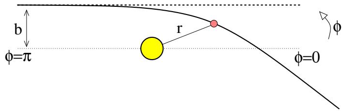
Figure 7. Light bending in the Schwarzschild metric.

We will solve the full equation (1.54) perturbatively in the small parameter

$$\tilde{\beta }=\frac{GM}{c^{2}b}$$

We then look for solutions of the form

$$u=u_0+\tilde{\beta }{u}_1+\dots$$

We start with the straight line solution $u_0=(1/b)$ sin $\varphi$ . At leading order, we then have

$$\frac{d^2{u}_1}{d{\varphi }^2}+u_1=\frac{3{\sin }^2\varphi }{b}=\frac{3(1-\cos 2\varphi )}{2b}$$

The general solution is

$$u_1=A\cos \varphi +B\sin \varphi +\frac{1}{2b}(3+\cos 2\varphi )$$

where the first two terms are the complimentary solution, with A and B integration constants. We pick them so that the initial trajectory at $\varphi =\pi$ agrees with the straight line $u_0$ . This holds if we choose $B=0$ and $A=2/b,$ so that $u_1\to 0$ as $\varphi \to \pi$ . To leading order in $\tilde{\beta }.$ , the solution is then

$$u=\frac{1}{b}\sin \varphi +\frac{GM}{2b^2{c}^2}(3+4\cos \varphi +\cos 2\varphi )$$

The question now is: at what angle does the particle escape to $r=\infty$ or , equivalently, $u=0?$ Before we made the correction this happened at $\varphi =0$ . Within our perturbative approach, we can approximate sin $\varphi \approx \varphi$ and cos $\varphi \approx 1$ to find that the particle escapes at

$$\varphi \approx -\frac{4GM}{b{c}^2}\text{\hspace{1em}(1.55)}$$

This light bending is known as gravitational lensing.

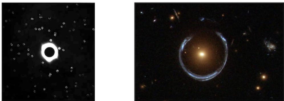
Figure 8. Gravitational lensing, as seen by Eddington’s 1919 eclipse expedition on the left. And as seen by the Hubble space telescope on the right.

For the Sun, $G{M}_{\odot }/c^2\approx 1.5$ km. If light rays just graze the surface, then the impact parameter b coincides with the radius of the Sun, $R_{\odot }\approx 7\times 10^5$ km. This gives a scattering angle of $\varphi \approx 8.6\times 10^{-5}$ radians, or $\varphi \approx 1.8^{\prime \prime }$

There is a difficulty in testing this prediction: things behind the Sun are rarely visible. However, Nature is kind to us because the size of the moon as seen in the sky is more or less the same as the size of the Sun. (This random coincidence would surely make our planet a popular tourist destination for alien hippies if only it wasn’t such a long way to travel.) This means that during a solar eclipse the light from the Sun is blocked, allowing us to measure the positions of stars whose light passes nearby the Sun. This can then be compared to the usual positions of these stars.

This measurement was first carried out in May 1919, soon after cessation of war, in two expeditions led by Arthur Eddington, one to the island of Principe and the other to Brazil. The data is shown in the figure above. In the intervening century, we have much more impressive evidence of light bending, in which clusters of galaxies distort the light from a background source, often revealing a distinctive ring-like pattern as shown in the right-hand figure.

Newtonian Scattering of Light

Before we claim success, we should check to see if the relativistic result (1.55) differs from the Newtonian prediction for light bending. Strictly speaking, there’s an ambiguity in the Newtonian prediction for the gravitational force on a massless particle. However, we can invoke the principle of equivalence which tells us that trajectories are independent of the mass. We then extrapolate this result, strictly derived for massive particles, to the massless case.

Figure 9. The scattering of light using Newtonian gravity.

Scattering under Newtonian gravity follows a hyperbola (1.43)

$$\frac{1}{r}=\frac{GM}{l^2}(1+e\cos \varphi )$$

with $e>1$ . The parameterisation of the trajectory is a little different from the relativistic result, as the light ray asymptotes to infinity at cos $\varphi =-1/e$ . For $e\gg 1$ , where the trajectory is close to a straight line, the asymptotes occur at $\varphi =\pm (\pi +\delta \varphi )$ as shown in Figure 9. The scattering angle is then 2δϕ. This is what we wish to compute.

Using (1.41), the speed of light along the trajectory is

$$\dot{r}=-l\frac{du}{d\varphi }=\frac{GM}{l}e\sin \varphi$$

This is one of the pitfalls of applying Newtonian methods to light bending: we will necessarily find that the speed of light changes as it moves in a gravitational field. The best we can do is ensure that light travels at speed c asymptotically, when cos $\varphi =-1/e$ and sin $\varphi =\sqrt{1-1/e^2}$ . This gives

$$c^2=\frac{G^2{M}^2}{l^2}(e^2-1)$$

Meanwhile the angular momentum is $l=bc$ , with b the impact parameter. Rearranging, we have

$$e^2=\frac{b^2{c}^4}{G^2{M}^2}+1\Rightarrow e\approx \frac{b{c}^2}{GM}$$

where, in the second equation, we have used the fact that we are interested in trajectories close to a straight line with $e\gg 1$ . As we mentioned above, the trajectory asymptotes to infinity at cos $\varphi =-1/e$ . This occurs at $\varphi =\pi /2+\delta \varphi$ and $\varphi =-\pi /2-\delta \varphi$ with

$$\delta \varphi \approx \frac{1}{e}\approx \frac{GM}{b{c}^2}$$

The resulting scattering angle is

$$2\delta \varphi \approx \frac{2GM}{b{c}^2}$$

We see that this is a factor of 2 smaller than the relativistic prediction (1.55)

The fact that relativistic light bending is twice as large as the Newtonian answer can be traced to the fact that both $g_{00}$ and $g_{rr}$ components of the Schwarzschild metric are non-vanishing. In some sense, the Newtonian result comes from the $g_{00}$ term, while the contribution from $g_{rr}$ is new. We’ll discuss this more in Section 5.1 where we explain how to derive Newtonian gravity from general relativity.

来源与版本

正文：英文 · OCR 机器稿 · 待校对

核对状态：OCR 机器稿 · 待校对

原书 PDF

来源版本：michaelmas-2019-source-20260923

来源 PDF SHA-256：3ba65dc61f22a69c7d5fdf3e8e1f641efbfa6cf49a44b3dcb0fd5367ba9fcf1c

OCR 来源 SHA-256：b7a5f3b8f7f5cc250cee6ca3e3930a672c39f068eeffa29106f5563d2cf79ec3

OCR 产物 SHA-256：ed78e176bec4e0ff89be44389a698c755518ca222de2b01dd6103a7bcb1fc564