1.2 Relativistic Particles

Having developed the tools to describe motion in curved space, our next step is to consider the relativistic generalization to curved spacetime. But before we get to this, we first need to see how to extend the Lagrangian method to be compatible with special relativity. An introduction to special relativity can be found in the lectures on Dynamics and Relativity.

1.2.1 A Particle in Minkowski Spacetime

Let’s start by considering a particle moving in Minkowski spacetime ${\mathbf{R}}^{1,3}$ . We’ll work with Cartesian coordinates $x^{\mu }=(ct,x,y,z)$ and the Minkowski metric

$${\eta }_{\mu \nu }=\mathrm{diag}(-1,+1,+1,+1)$$

The distance between two neighbouring points labelled by $x^{\mu }$ and $x^{\mu }+d{x}^{\mu }$ is then given by

$$d{s}^2={\eta }_{\mu \nu }d{x}^{\mu }d{x}^{\nu }$$

Pairs of points with $d{s}^2<0$ are said to be timelike separated; those for which $d{s}^2>0$ are spacelike separated; and those for which $d{s}^2=0$ are said to be lightlike separated or, more commonly, null.

Consider the path of a particle through spacetime. In the previous section, we labelled positions along the path using the time coordinate t for some inertial observer. But to build a relativistic description of the particle motion, we want time to sit on much the same footing as the spatial coordinates. For this reason, we will introduce a new parameter – let’s call it $\sigma -$ which labels where we are along the worldline of the trajectory. For now it doesn’t matter what parameterisation we choose; we will only ask that $\sigma$ increases monotonically along the trajectory. We’ll label the start and end points of the trajectory by ${\sigma }_1$ and ${\sigma }_2$ respectively, with $x^{\mu }({\sigma }_1)=x_{\mathrm{initial}}^{\mu }$ and $x^{\mu }({\sigma }_2)=x_{\mathrm{final}}^{\mu }$

The action for a relativistic particle has a nice geometric interpretation: it extremises the distance between the starting and end points in Minkowski space. A particle with rest mass m follows a timelike trajectory, for which any two points on the curve have $d{s}^2<0$ . We therefore take the action to be

$$\begin{array}{rl}& S=-mc{\int }_{x_{\mathrm{initial}}}^{x_{\mathrm{final}}}\sqrt{-d{s}^2}\\ & =-mc{\int }_{{\sigma }_1}^{{\sigma }_2}d\sigma \sqrt{-{\eta }_{\mu \nu }\frac{d{x}^{\mu }}{d\sigma }\frac{d{x}^{\nu }}{d\sigma }}\end{array}\text{\hspace{1em}(1.13)}$$

The coefficients in front ensure that the action has dimensions [S] = Energy × Time as it should. (The action always has the same dimensions as ℏ. If you work in units with $\hslash =1$ then the action should be dimensionless.)

The action (1.13) has two different symmetries, with rather different interpretations.

• Lorentz Invariance: Recall that a Lorentz transformation is a rotation in spacetime. This acts as

$$x^{\mu }\to {\Lambda }_{\rho }^{\mu }{x}^{\rho }\text{\hspace{1em}(1.14)}$$

where the matrix ${\Lambda }_{\nu }^{\mu }$ obeys ${\Lambda }_{\rho }^{\mu }{\eta }_{\mu \nu }{\Lambda }_{\sigma }^{\nu }={\eta }_{\rho \sigma }$ , which is the definition of a Lorentz transformation, encompassing both rotations in space and boosts. Equivalently, $\Lambda \in O(1,3)$ . This is a symmetry in the sense that if we find a solution to the equations of motion, then we can act with a Lorentz transformation to generate a new solution.

• Reparameterisation invariance: We introduced σ as an arbitrary parameterisation of the path. But we don’t want the equations of motion to depend on this choice. Thankfully all is good, because the action itself does not depend on the choice of parameterisation. To see this, suppose that we picked a different parameterisation of the path, $\tilde{\sigma },$ related to the first parameterisation by a monotonic function $\tilde{\sigma }(\sigma )$ Then we could equally as well construct an action $\tilde{S}$ using this new parameter, given by

$$\begin{array}{rl}& \tilde{S}=-mc{\int }_{{\tilde{\sigma }}_1}^{{\tilde{\sigma }}_2}d\tilde{\sigma }\sqrt{-{\eta }_{\mu \nu }\frac{d{x}^{\mu }}{d\tilde{\sigma }}\frac{d{x}^{\nu }}{d\tilde{\sigma }}}\\ & =-mc{\int }_{{\sigma }_1}^{{\sigma }_2}d\sigma \frac{d\tilde{\sigma }}{d\sigma }\sqrt{-{\eta }_{\mu \nu }\frac{d{x}^{\mu }}{d\sigma }\frac{d{x}^{\nu }}{d\sigma }{\left(\frac{d\sigma }{d\tilde{\sigma }}\right)}^2}\\ & =S\end{array}$$

As promised, the action takes the same form regardless of whether we choose to parameterise the path in terms of $\sigma$ or $\tilde{\sigma }$ . This is reparameterisation invariance. This is not a symmetry, in the sense that it does not generate new solutions from old ones. Instead, it is a redundancy in the way we describe the system. It is similar to the gauge “symmetry” of Maxwell and Yang-Mills theory which, despite the name, is also a redundancy rather than a symmetry.

It is hard to overstate the importance of the concept of reparameterisation invariance. A major theme of these lectures is that our theories of physics should not depend on the way we choose to parameterise them. We’ll see this again when we come to describe the field equations of general relativity. For now, we’ll look at a couple of implications of reparameterisation on the worldline.

Proper Time

Because the action is independent of the parameterisation of the worldline, the value of the action evaluated between two points on a given path has an intrinsic meaning. We call this value proper time. For a given path $x^{\mu }({\sigma }^{\prime })$ , the proper time between two points, say ${\sigma }^{\prime }=0$ and ${\sigma }^{\prime }=\sigma$ , is

$$\tau (\sigma )=\frac{1}{c}{\int }_0^{\sigma }d{\sigma }^{\prime }\sqrt{-g_{\mu \nu }(x)\frac{d{x}^{\mu }}{d{\sigma }^{\prime }}\frac{d{x}^{\nu }}{d{\sigma }^{\prime }}}\text{\hspace{1em}(1.15)}$$

From our first foray into Special Relativity, we recognise this as the time experienced by the particle itself.

Identifying the action with the proper time means that the particle takes a path that extremises the proper time. In Minkowski space, it is simple to check that the proper time between two timelike-separated points is maximised by a straight line, a fact known as the twin paradox.

1.2.2 Why You Get Old

There’s a crucial difference between moving in Euclidean space and moving in Minkowski spacetime. You’re not obliged to move in Euclidean space. You can just stop if you want to. In contrast, you can never stop moving in a timelike direction in Minkowski spacetime. You will, sadly, always be dragged inexorably towards the future.

Any relativistic formulation of particle mechanics must capture this basic fact. To see how it arises from the action (1.13), we can compute the momentum conjugate to $x^{\mu }$

$$p_{\mu }=\frac{dL}{d{\dot{x}}^{\mu }}\text{\hspace{1em}(1.16)}$$

with ${\dot{x}}^{\mu }=d{x}^{\mu }/d\sigma$ . For the action $L=-mc\sqrt{-{\eta }_{\mu \nu }{\dot{x}}^{\mu }{\dot{x}}^{\nu }}$ , we have

$$p_{\mu }=mc\frac{{\eta }_{\mu \nu }{\dot{x}}^{\nu }}{\sqrt{-{\eta }_{\rho \sigma }{\dot{x}}^{\rho }{\dot{x}}^{\sigma }}}=-\frac{m^2{c}^2}{L}{\eta }_{\mu \nu }{\dot{x}}^{\nu }\text{\hspace{1em}(1.17)}$$

But not all four components of the momentum are independent. To see this, we need only compute the square of the 4-momentum to find

$$p\cdot p\equiv {\eta }_{\mu \nu }{p}^{\mu }{p}^{\nu }=\frac{m^4{c}^4}{L^2}{\eta }_{\mu \nu }{\dot{x}}^{\mu }{\dot{x}}^{\nu }=-m^2{c}^2\text{\hspace{1em}(1.18)}$$

Rearranging gives

$$(p^0{)}^2={\mathbf{p}}^2+m^2{c}^2$$

In particular, we see that we must have $p^0\ne 0;$ : the particle is obliged to move in the time direction.

Part of this story is familiar. The condition (1.18) is closely related to the usual condition on the 4-momentum that we met in our earlier lectures on Special Relativity. There, we defined the 4-velocity $U^{\mu }$ and 4-momentum $P^{\mu }$ as

$$U^{\mu }=\frac{d{x}^{\mu }}{d\tau }\mathrm{and}{P}^{\mu }=m\frac{d{x}^{\mu }}{d\tau }$$

This is a special case of (1.16), where we choose to parameterise the worldline by the proper time $\tau$ itself. The definition of the proper time (1.15) means that $d\tau /d\sigma =$ $-L/m{c}^2$ . Comparing to the canonical momentum (1.17), we see that it coincides with the older definition above: $P^{\mu }\equiv p^{\mu }$

However, part of this story is likely unfamiliar. Viewed from the perspective of classical dynamics, it is perhaps surprising to see that the momenta $p^{\mu }$ are not all independent. After all, this didn’t arise in any of the examples of Lagrangians that we met in our previous course on Classical Dynamics. This novel feature can be traced to the existence of reparameterisation invariance, meaning that there was a redundancy in our original description. Indeed, whenever theories have such a redundancy there will be some constraint analogous to (1.18). (In the context of electromagnetism, this constraint is called Gauss law.)

There is another way to view this. The relativistic action (1.13) appears to have four dynamical degrees of freedom, $x^{\mu }(\sigma )$ . This should be contrasted with the three degrees of freedom $x^i(t)$ in the non-relativistic action (1.5). Yet the number of degrees of freedom is one of the most basic ways to characterise a system, with physical consequences such as the heat capacity of gases. Why should we suddenly increase the number of degrees of freedom just because we want our description to be compatible with special relativity? The answer is that, because of reparameterisation invariance, not all four degrees of freedom $x^{\mu }$ are physical. To see this, suppose that you solve the equations of motion to find the path $x^{\mu }(\sigma )$ (as we will do shortly). In most dynamical systems, each of these four functions would tell you something about the physical trajectory. But, for us, reparameterisation invariance means that there is no actual information in the value of $\sigma$ . To find the physical path, we should eliminate $\sigma$ to find the relationship between the $x^{\mu }$ . The net result is that the relativistic system only has three physical degrees of freedom after all.

As an example, we are perfectly at liberty to choose the parameterisation of the path to coincide with the time t for some inertial observer: $\sigma =t$ . The action (1.13) then becomes

$$S=-m{c}^2{\int }_{t_1}^{t_2}dt\sqrt{1-\frac{{\dot{\mathbf{x}}}^2}{c^2}}\text{\hspace{1em}(1.19)}$$

where here $\dot{\mathbf{x}}=d\mathbf{x}/dt$ . This is the action for a relativistic particle in some particular inertial frame, which exhibits the famous factor

$$\gamma =\frac{1}{\sqrt{1-{\dot{\mathbf{x}}}^2/c^2}}$$

that is omnipresent in formulae in special relativity. We now see clearly that the action has only three degrees of freedom, $\mathbf{x}(t)$ . However, the price we’ve paid is that the Lorentz invariance (1.14) is now rather hidden, since space x and time t sit on very different footing.

1.2.3 Rediscovering the Forces of Nature

So far, we’ve only succeeded in writing down the action for a free relativistic particle (1.13). We would now like to add some extra terms to the action to describe a force acting on the particle. In the non-relativistic context, we do this by adding a potential

$$S_{\mathrm{non}-\mathrm{rel}}=\int dt\left[\frac{m}{2}{\dot{\mathbf{x}}}^2-V(\mathbf{x})\right]$$

However, now we want to write down an action for a relativistic particle that depends on $x^{\mu }(\sigma )$ . But it’s crucial that we retain reparameterisation invariance, since we want to keep the features that this brings. This greatly limits the kind of terms that we can add to the action. It turns out that there are two, different ways to introduce forces that preserve our precious reparameterisations.

Rediscovering Electromagnetism

Rather than jumping straight into the reparameterisation invariant action (1.13), we instead start by modifying the action (1.19). We’ll then try to guess a reparameterisation invariant form which gives the answer we want. To this end, we consider

$$S_1={\int }_{t_1}^{t_2}dt\left[-m{c}^2\sqrt{1-\frac{{\dot{\mathbf{x}}}^2}{c^2}}-V(\mathbf{x})\right]$$

and ask: how can this come from a reparameterisation invariant action?

We can’t just add a term R dσ $V(x)$ to the relativistic action (1.13); this is not invariant under reparameterisations. To get something that works, we have to find a way to cancel the Jacobian factor that comes from reparameterisations of the dσ measure. One option that we could explore is to introduce a term linear in ${\dot{x}}^{\mu }$ . But then, to preserve Lorentz invariance, we need to contract the $\mu$ index on ${\dot{x}}^{\mu }$ with something. This motivates us to introduce four functions of the spacetime coordinates $A_{\mu }(x)$ . We then write the action

$$S_1={\int }_{{\sigma }_1}^{{\sigma }_2}d\sigma \left[-mc\sqrt{-{\eta }_{\mu \nu }\frac{d{x}^{\mu }}{d\sigma }\frac{d{x}^{\nu }}{d\sigma }}-q{A}_{\mu }(x){\dot{x}}^{\mu }\right]\text{\hspace{1em}(1.20)}$$

where $q$ is some number, associated to the particle, that characterises the strength with which it couples to the new term $A_{\mu }(x)$ . It’s simple to check that the action (1.20) does indeed have reparameterisation invariance.

To understand the physics of this new term, we again pick the worldline parameter to coincide with the time of some inertial observer, $\sigma =t$ so that $d{x}^0/d\sigma =c$ . If we write $A_{\mu }(x)=(\varphi (x)/c,\mathbf{A}(x))$ ), then we find

$$S_1={\int }_{{\sigma }_1}^{{\sigma }_2}d\sigma \left[-m{c}^2\sqrt{1-\frac{{\dot{\mathbf{x}}}^2}{c^2}}-q\varphi (x)-q\mathbf{A}(x)\cdot \dot{\mathbf{x}}\right]$$

We see that the $A_0$ term gives us a potential $V(x)=q\varphi (x)$ of the kind we wanted. But Lorentz invariance means that this is accompanied by an additional $\mathbf{A}\cdot \dot{\mathbf{x}}$ term. We have, of course, met both of these terms previously: they describe a particle of electric charge q moving in the background of an electromagnetic field described by gauge potentials $\varphi (x)$ and $\mathbf{A}(x)$ . In other words, we have rediscovered the Lorentz force law of electromagnetism.

There is a slight generalisation of this argument, in which the particle carries some extra internal degrees of freedom, that results in the mathematical structure of Yang-Mills, the theory that underlies the weak and strong nuclear force. You can read more about this in the lecture notes on Gauge Theory.

Rediscovering Gravity

To describe the force of gravity, we must make a rather different modification to our action. This time we consider the generalisation of (1.19) given by the action

$$S_2={\int }_{t_1}^{t_2}dt\left[-m{c}^2\sqrt{1+\frac{2\Phi (\mathbf{x})}{c^2}-\frac{{\dot{\mathbf{x}}}^2}{c^2}}\right]\text{\hspace{1em}(1.21)}$$

If we Taylor expand the square-root, assuming that $|\dot{\mathbf{x}}|\ll c^2$ and that $2\Phi (\mathbf{x})\ll c^2,$ 2 then the leading terms give

$$S_2={\int }_{t_1}^{t_2}dt\left[-m{c}^2+\frac{m}{2}{\dot{\mathbf{x}}}^2-m\Phi (\mathbf{x})+\dots \right]\text{\hspace{1em}(1.22)}$$

The first term is an irrelevant constant. (It is the rest mass energy of the particle.) But the next two terms describe the non-relativistic motion of a particle moving in a potential $V(\mathbf{x})=m\Phi (\mathbf{x})$

Why should we identify this potential with the force of gravity, rather than some other random force? It’s because the strength of the force is necessarily proportional to the mass m of the particle, which shows up as the coefficient in the $m\Phi (\mathbf{x})$ term. This is the defining property of gravity.

In fact, something important but subtle has emerged from our simple discussion: the same mass m appears in both the kinetic term and the potential term. In the framework of Newtonian mechanics there is no reason that these coefficients should be the same. Indeed, careful treatments refer to the coefficient of the kinetic term as the inertial mass $m_I$ and the coefficient of the potential term as the gravitational mass $m_G$ It is then an experimentally observed fact that

$$m_I=m_G\text{\hspace{1em}(1.23)}$$

to astonishing accuracy (around $10^{-13})$ . This is known as the equivalence principle. But our simple-minded discussion above has offered a putative explanation for the equivalence principle, since the mass m sits in front of the entire action (1.21), ensuring that both terms have the same origin.

An aside: you might wonder why the function $\Phi (x)$ does not scale as, say, $1/m$ , in which case the potential that arises in (1.22) would appear to be independent of $m.$ This is not allowed. This is because the mass m is a property of the test particle whose motion we’re describing. Meanwhile the potential $\Phi (x)$ is some field set up by the background sources, and should be independent of $m,$ just as $A_{\mu }(x)$ is independent of the charge $q$ of the test particle.

The equality (1.23) is sometimes called the weak equivalence principle. A stronger version, known as the Einstein equivalence principle says that in any metric there exist local inertial frames. This is the statement that you can always find coordinates so that, in some small patch, the metric looks like Minkowski space, and there is no way to detect the effects of the gravitational field. We will describe this more below and again in Section 3.3.2.

Finally, we ask: how can we write down a reparameterisation invariant form of the action (1.21)? To answer this, note that the 1 in $\sqrt{1+\dots }$ came from the ${\eta }_{00}$ term in the action. If we want to turn this into $1+2\Phi (\mathbf{x})/c^2$ , then we should promote ${\eta }_{00}$ to a function of x. But if we’re going to promote ${\eta }_{00}$ to a function, we should surely do the same to all metric components. This means that we introduce a curved spacetime metric

$$d{s}^2=g_{\mu \nu }(x)d{x}^{\mu }d{x}^{\nu }$$

The metric is a symmetric 4×4 matrix, which means that it is specified by 10 functions. We can then write down the reparameterisation invariant action

$$S_2=-mc{\int }_{{\sigma }_1}^{{\sigma }_2}d\sigma \sqrt{-g_{\mu \nu }(x)\frac{d{x}^{\mu }}{d\sigma }\frac{d{x}^{\nu }}{d\sigma }}$$

This describes a particle moving in curved spacetime.

In general, the components of the metric will be determined by the Einstein field equations. This is entirely analogous to the way in which the gauge potential $A_{\mu }(x)$ in (1.20) is determined by the Maxwell equation. We will describe the Einstein equations in Section 4. However, even before we get to the Einstein equations, the story above tells us that, for weak gravitational fields where the Newtonian picture is valid, we should identify

$$g_{00}(x)\approx -\left(1+\frac{2\Phi (x)}{c^2}\right)\text{\hspace{1em}(1.24)}$$

where $\Phi (x)$ is the Newtonian gravitational field.

1.2.4 The Equivalence Principle

A consequence of the weak equivalence principle (1.23) is that it’s not possible to tell the difference between constant acceleration and a constant gravitational field. Suppose, for example, that you one day wake up to find yourself trapped inside a box that looks like an elevator. The equivalence principle says that there’s no way tell whether you are indeed inside an elevator on Earth, or have been captured by aliens and are now in the far flung reaches of the cosmos in a spaceship, disguised as an elevator, and undergoing constant acceleration. (Actually there are two ways to distinguish between these possibilities. One is common sense. The other is known as tidal forces and will be described below.)

Conversely, if you wake in the elevator to find yourself weightless, the equivalence principle says that there is no way to tell whether the engines on your spaceship have turned themselves of, leaving you floating in space, or whether you are still on Earth, plummeting towards certain death. Both of these are examples of inertial frames.

We can see how the equivalence principle plays out in more detail in the framework of spacetime metrics. We will construct a set of coordinates adapted to a uniformly accelerating observer. We’ll see that, in these coordinates, the metric takes the form (1.24) but with a linear gravitational potential Φ of the kind that we would invoke for a constant gravitational force.

First we need to determine the trajectory of a constantly accelerating observer. This was a problem that we addressed already in our first lectures on Special Relativity (see Section 7.4.6 of those notes). Here we give a different, and somewhat quicker, derivation.

We will view things from the perspective of an inertial frame, with coordinates $(ct,x,y,z)$ . The elevator will experience a constant acceleration a in the x direction. We want to know what this looks like in the inertial frame; clearly the trajectory is not just $x=\frac{1}{2}a{t}^2$ since this would soon exceed the speed of light. Instead we need to be more careful.

Recall that if we do a boost by $v_1$ , followed by a boost by $v_2$ , the resulting velocity is

$$v=\frac{v_1+v_2}{1+v_1{v}_2/c^2}$$

This motivates us to define the rapidity $\phi ,$ defined in terms of the velocity v by

$$v=c\tanh \phi$$

The rapidity has the nice property that is adds linearly under successive boosts: a boost ${\phi }_1$ followed by a boost ${\phi }_2$ is the same as a boost $\phi ={\phi }_1+{\phi }_2$

A constant acceleration means that the rapidity increases linearly in time, where here “time” is the accelerating observer’s time, τ . We have $\phi =a\tau /c$ and so, from the perspective of the inertial frame, the velocity of the constantly-accelerating elevator

$$v(\tau )=\frac{dx}{dt}=c\tanh \left(\frac{a\tau }{c}\right)$$

To determine the relationship between the observer’s time and the time t in the inertial frame, we use

$$\frac{dt}{d\tau }=\gamma (\tau )=\sqrt{\frac{1}{1-v^2/c^2}}=\cosh \left(\frac{a\tau }{c}\right)\Rightarrow t=\frac{c}{a}\sinh \left(\frac{a\tau }{c}\right)$$

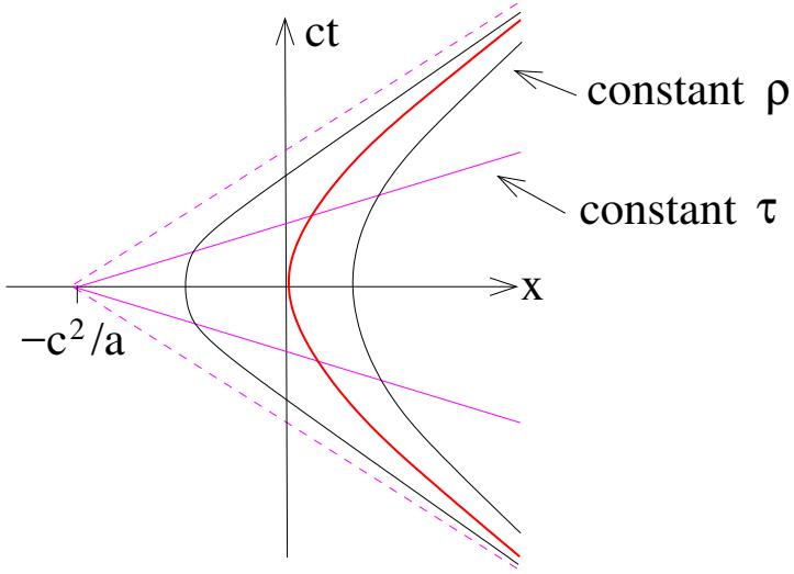
Figure 1. A coordinate system for a uniformly accelerating observer.

where we’ve chosen the integration constant so that $\tau =0$ corresponds to $t=0$ . Then, to determine the distance travelled in the inertial frame, we use

$$v(\tau )=\frac{dx}{dt}=\frac{dx}{d\tau }\frac{d\tau }{dt}\Rightarrow \frac{dx}{d\tau }=c\sinh \left(\frac{a\tau }{c}\right)\Rightarrow x=\frac{c^2}{a}\cosh \left(\frac{a\tau }{c}\right)-\frac{c^2}{a}$$

where this time we’ve chosen the integration constant so that the trajectory passes through the origin. The resulting trajectory is a hyperbola in spacetime, given by

$${\left(x+\frac{c^2}{a}\right)}^2-c^2{t}^2=\frac{c^4}{a^2}$$

This trajectory is shown in red in Figure 1. As $\tau \to \pm \infty$ , the trajectory asymptotes to the straight lines $ct=\pm (x+c^2/a)$ . These are the dotted lines shown in the figure.

Now let’s consider life from the perspective of guy in the accelerating elevator. What are the natural coordinates that such an observer would use to describe events elsewhere in spacetime? Obviously, for events that happen on his own worldline, we can use the proper time τ . But we would like to extend the definition to assign a time to points in the whole space. Furthermore, we would like to introduce a spatial coordinate, $\rho ,$ so that the elevator sits at $\rho =0$ . How to do this?

There is, it turns out, a natural choice of coordinates. First, we draw straight lines connecting the point $(ct,x)=(0,-c^2/a)$ to the point on the trajectory labelled by $\tau$ and declare that these are lines of constant $\tau ;$ these are the pink lines shown in the figure. Next we note that, for any given ${\tau }_{:}$ there is a Lorentz transformation that maps the x-axis to the pink line of constant $\tau$ . We can use this to define the spatial coordinate $\rho .$ The upshot is that we have a map between coordinates $(ct,x)$ in the inertial frame and coordinates $(c\tau ,\rho )$ in the accelerating frame given by

$$\begin{array}{rl}& ct=\left(\rho +\frac{c^2}{a}\right)\sinh \left(\frac{a\tau }{c}\right)\\ & x=\left(\rho +\frac{c^2}{a}\right)\cosh \left(\frac{a\tau }{c}\right)-\frac{c^2}{a}\end{array}\text{\hspace{1em}(1.25)}$$

As promised, the line $\rho =0$ coincides with the trajectory of the accelerating observer. Moreover, lines of constant $\rho \ne 0$ are also hyperbolae.

The coordinates $(c\tau ,\rho )$ do not cover all of Minkowski space, but only the right-hand quadrant as shown in Figure 1. This reflects the fact that signals from some regions will never reach the guy in the elevator. This is closely related to the idea of horizons in general relativity, a topic we’ll look explore more closely in later sections.

Finally, we can look at the metric experienced by the accelerating observer, using coordinates $\rho$ and $\tau$ . We simply substitute the transformation (1.25) into the Minkowski metric to find

$$d{s}^2=-c^{2}d{t}^2+d{x}^2+d{y}^2+d{z}^2=-{\left(1+\frac{a\rho }{c^2}\right)}^2{c}^{2}d{\tau }^2+d{\rho }^2+d{y}^2+d{z}^2$$

This is the metric of (some part of ) Minkowski space, now in coordinates adapted to an accelerating observer. These are known as Kottler-M¨oller coordinates. (They are closely related to the better known Rindler coordinates. We’ll see Rindler space again in Section 6.1.2 when we study the horizon of black holes. ) The spatial part of the metric remains flat, but the temporal component is given by

$$g_{00}=-{\left(1+\frac{a\rho }{c^2}\right)}^2=-\left(1+\frac{2a\rho }{c^2}+\dots \right)$$

where the $\cdot \cdot \cdot$ is simply $a^2{\rho }^2/c^4$ , but we’ve hidden it because it is sub-leading in $1/c^2$ If we compare this metric with the expectation (1.24), we see that the accelerated observer feels an effective gravitational potential given by

$$\Phi (\rho )=a\rho$$

This is the promised manifestation of the equivalence principle: from the perspective of an uniformly accelerating observer, the acceleration feels indistinguishable from a linearly increasing gravitational field, corresponding to a constant gravitational force.

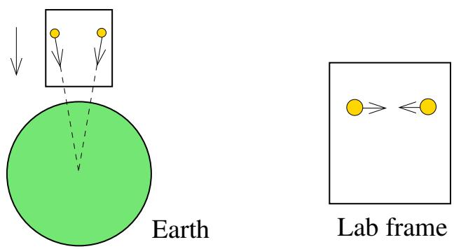
Figure 2. The bad news is that you were, in fact, plummeting to your death after all. This is shown on the left (not to scale). The good news is that you get to measure a tidal force on the way down. This is shown on the right.

The Einstein Equivalence Principle

The weak equivalence principle tells us that uniform acceleration is indistinguishable from a uniform gravitational field. In particular, there is a choice of inertial frame (i.e. free-fall) in which the effect of the gravitational field vanishes. But what if the gravitational field is non-uniform?

The Einstein equivalence principle states that there exist local inertial frames, in which the effects of any gravitational field vanish. Mathematically, this means that there is always a choice of coordinates — essentially those experienced by a freely falling observer – which ensures that the metric $g_{\mu \nu }$ looks like Minkowski space about a given point. (We will exhibit these coordinates and be more precise about their properties in Section 3.3.2.) The twist to the story is that if the metric looks like Minkowski space about one point, then it probably won’t look like Minkowski space about a different point. This means that if you can do experiments over an extended region of space, then you can detect the presence of non-uniform gravitational field.

To illustrate this, let’s return to the situation in which you wake, weightless in an elevator, trying to figure out if you’re floating in space or plummeting to your death. How can you tell?

Well, you could wait and find out. But suppose you’re impatient. The equivalence principle says that there is no local experiment you can do that will distinguish between these two possibilities. But there is a very simple “non-local” experiment: just drop two test masses separated by some distance. If you’re floating in space, the test masses will simply float there with you. Similarly, if you’re plummeting towards your death then the test masses will plummet with you. However, they will each be attracted to the centre of the Earth which, for two displaced particles, is in a slightly different direction as shown in Figure 2. This means that the trajectories followed by the particles will slightly converge. From your perspective, this will mean that the two test masses will get closer. This is not due to their mutual gravitational attraction. (The fact they’re test masses means we’re ignoring this). Instead, it is an example of a tidal force that signifies you’re sitting in a non-uniform gravitational field. We will meet the mathematics behind these tidal forces in Section 3.3.4.

1.2.5 Gravitational Time Dilation

Even before we solve the Einstein equations, we can still build some intuition for the spacetime metric. As we’ve seen, for weak gravitational fields $\Phi (\mathbf{x})$ , we should identify the temporal component of the metric as

$$g_{00}(x)=1+\frac{2\Phi (x)}{c^2}\text{\hspace{1em}(1.26)}$$

This is telling us something profound: there is a connection between time and gravity.

To be concrete, we’ll take the Newtonian potential that arises from a spherical object of mass M,

$$\Phi (r)=-\frac{GM}{r}$$

The resulting shift in the spacetime metric $g_{00}$ means that an observer sitting at a fixed distance r will measure a time interval,

$$d{\tau }^2=g_{00}d{t}^2=\left(1-\frac{2GM}{r{c}^2}\right)d{t}^2$$

This means that if an asymptotic observer, at $r\to \infty$ , measures time t, then an observer at distance r will measure time T given by

$$T(r)=t\sqrt{1-\frac{2GM}{r{c}^2}}$$

We learn that time goes slower in the presence of a massive, gravitating object.

We can make this more quantitative. Consider two observers. The first, Alice, is relaxing with a picnic on the ground at radius $r_A$ . The second, Bob, is enjoying a romantic trip for one in a hot air balloon, a distance $r_B=r_A+\Delta r$ higher. The time measured by Bob is

$$\begin{array}{rl}& T_B=t\sqrt{1-\frac{2GM}{(r_A+\Delta r)c^2}}\approx t\sqrt{1-\frac{2GM}{r_A{c}^2}+\frac{2GM\Delta r}{r_A^2{c}^2}}\\ & \approx t\sqrt{1-\frac{2GM}{r_A{c}^2}}\left(1+\frac{GM\Delta r}{r_A^2{c}^2}\right)=T_A\left(1+\frac{GM\Delta r}{r_A^2{c}^2}\right)\end{array}$$

where we’ve done a double expansion, assuming both $\Delta r\ll r_A$ and $2GM/r_A{c}^2\ll 1$ If the hot air balloon flies a distance $\Delta r=1000$ m above the ground then, taking the radius of the Earth to be $r_A\approx 6000$ km, the difference in times is of order $10^{-12}$ . This means that, over the course of a day, Bob ages by an extra 10⁻⁸ seconds or so.

This effect was first measured by Hafele and Keating in the 1970s by flying atomic clocks around the world on commercial airlines, and has since been repeated a number of times with improved accuracy. In all cases the resultant time delay, which in the experiments includes effects from both special and general relativity, was in agreement with theoretical expectations.

The effect is more pronounced in the vicinity of a black hole. We will see in Section 1.3 that the closest distance that an orbiting planet can come to a black hole is $r=3GM/c^2$ (Such orbits are necessarily highly elliptical.) In this case, someone on the planet experiences time at the rate $T=\sqrt{1/3}t\approx 0.6t$ , compared to an asymptotic observer at $t\to \infty$ . This effect, while impressive, is unlikely to make a really compelling science fiction story. For more dramatic results, our bold hero would have to fly her spaceship close to the Schwarzschild radius $R_s=2GM/c^2$ , later returning to $r\to \infty$ to find herself substantially younger than the friends and family she left behind.

Gravitational Redshift

There is another measurable consequence of the gravitational time dilation. To see this, let’s return to Alice on the ground and Bob, above, in his hot air balloon. Bob is kind of annoying and starts throwing peanuts at Alice. He throws peanuts at time intervals $\Delta T_B$ . Alice receives these peanuts (now travelling at considerable speed) at time intervals $\Delta T_A$ where, as above,

$$\Delta T_A=\sqrt{\frac{1+2\Phi (r_A)/c^2}{1+2\Phi (r_B)/c^2}}\Delta T_B\approx \left(1+\frac{\Phi (r_A)}{c^2}-\frac{\Phi (r_B)}{c^2}\right)\Delta T_B$$

We have $r_A<r_B$ , so $\Phi (r_A)<\Phi (r_B)<0$ and, hence, $\Delta T_A<\Delta T_B$ . In other words, Alice receives the peanuts at a higher frequency than Bob threw them.

The story above doesn’t only hold for peanuts. If Bob shines light down at Alice with frequency ${\omega }_B\sim 1/\Delta T_B$ , then Alice will receive it at frequency ${\omega }_A$ given by

$${\omega }_A\approx {\left(1+\frac{\Phi (r_A)}{c^2}-\frac{\Phi (r_B)}{c^2}\right)}^{-1}{\omega }_B$$

This is a higher frequency, ${\omega }_A>{\omega }_B$ , or shorter wavelength. We say that the light has been blueshifted. In contrast, if Alice shines light up at Bob, then the frequency decreases, and the wavelength is stretched. In this case, we say that the light has been redshifted as it escapes the gravitational pull. This effect was measured for the first time by Pound and Rebka in 1959, providing the first earthbound precision test of general relativity.

There is a cosmological counterpart of this result, in which light is redshifted in a background expanding space. You can read more about this in the lectures on Cosmology.

1.2.6 Geodesics in Spacetime

So far, we have focussed entirely on the actions describing particles, and have yet to write down an equation of motion, let alone solve one. Now it’s time to address this.

We work with the relativistic action for a particle moving in spacetime

$$S=-mc{\int }_{{\sigma }_1}^{{\sigma }_2}d\sigma L\text{ with }L=\sqrt{-g_{\mu \nu }(x){\dot{x}}^{\mu }{\dot{x}}^{\nu }}\text{\hspace{1em}(1.27)}$$

with ${\dot{x}}^{\mu }=d{x}^{\mu }/d\sigma$ . This is similar to the non-relativistic action that we used in Section 1.1.1 when we first introduced geodesics. It differs by the square-root factor. As we now see, this introduces a minor complication.

To write down Euler-Lagrange equations, we first compute

$$\frac{\partial L}{\partial x^{\rho }}=-\frac{1}{2L}\frac{\partial g_{\mu \nu }}{\partial x^{\rho }}{\dot{x}}^{\mu }{\dot{x}}^{\nu }\mathrm{and}\frac{\partial L}{\partial {\dot{x}}^{\rho }}=-\frac{1}{L}{g}_{\rho \nu }{\dot{x}}^{\nu }$$

The equations of motion are then

$$\frac{d}{d\sigma }\left(\frac{\partial L}{\partial {\dot{x}}^{\rho }}\right)-\frac{\partial L}{\partial x^{\rho }}=0\Rightarrow \frac{d}{d\sigma }\left(\frac{1}{L}{g}_{\rho \nu }{\dot{x}}^{\nu }\right)-\frac{1}{2L}\frac{\partial g_{\mu \nu }}{\partial x^{\rho }}{\dot{x}}^{\mu }{\dot{x}}^{\nu }=0$$

This is almost the same as the equations that led us to the geodesics in Section 1.1.1. There is just one difference: the differentiation $d/d\sigma$ can hit the $1/L$ , giving an extra term beyond what we found previously. This can be traced directly to the fact we have a square-root in our original action.

Following the same steps that we saw in Section 1.1.1, and relabelling the indices, the equation of motion can be written as

$$g_{\mu \rho }{\ddot{x}}^{\rho }+\frac{1}{2}\left(\frac{\partial g_{\mu \rho }}{\partial x^{\nu }}+\frac{\partial g_{\mu \nu }}{\partial x^{\rho }}-\frac{\partial g_{\nu \rho }}{\partial x^{\mu }}\right){\dot{x}}^{\nu }{\dot{x}}^{\rho }=\frac{1}{L}\frac{dL}{d\sigma }{g}_{\mu \rho }{\dot{x}}^{\rho }\text{\hspace{1em}(1.28)}$$

This is the relativistic version of the geodesic equation (1.6). We see that the squareroot factor in the action results in the extra term on the right-hand side.

Life would be much nicer if there was some way to ignore this extra term. This would be true if, for some reason, we could set

$$\frac{dL}{d\sigma }\stackrel{?}{=}0$$

Happily, this is within our power. We simply need to pick a choice of parameterisation of the worldline to make it hold! All we have to do is figure out what parameterisation makes this work.

In fact, we’ve already met the right choice. Recall that the proper time $\tau (\sigma )$ is defined as (1.15)

$$c\tau (\sigma )={\int }_0^{\sigma }d{\sigma }^{\prime }L({\sigma }^{\prime })={\int }_0^{\sigma }d{\sigma }^{\prime }\sqrt{-g_{\mu \nu }(x)\frac{d{x}^{\mu }}{d{\sigma }^{\prime }}\frac{d{x}^{\nu }}{d{\sigma }^{\prime }}}\text{\hspace{1em}(1.29)}$$

This means that, by construction,

$$c\frac{d\tau }{d\sigma }=L(\sigma )$$

If we then choose to parameterise the path by τ itself, the Lagrangian is

$$L(\tau )=\sqrt{-g_{\mu \nu }(x)\frac{d{x}^{\mu }}{d\tau }\frac{d{x}^{\nu }}{d\tau }}=\frac{d\sigma }{d\tau }\sqrt{-g_{\mu \nu }(x)\frac{d{x}^{\mu }}{d\sigma }\frac{d{x}^{\nu }}{d\sigma }}=c$$

The upshot of this discussion is that if we parameterise the worldline by proper time then $L=c$ is a constant and, in particular, $dL/d\tau =0$ . In fact this holds for any parameter related to proper time by

$$\tilde{\tau }=a\tau +b$$

with a and b constants. These are said to be affine parameters of the worldline.

Whenever we pick such an affine parameter to label the worldline of a particle, the right-hand side of the equation of motion (1.28) vanishes. In this case, we are left with the obvious extension of the geodesic equation (1.7) to curved spacetime

$$\frac{d^2{x}^{\mu }}{d{\tilde{\tau }}^2}+{\Gamma }_{\nu \rho }^{\mu }\frac{d{x}^{\nu }}{d\tilde{\tau }}\frac{d{x}^{\rho }}{d\tilde{\tau }}=0\text{\hspace{1em}(1.30)}$$

where the Christoffel symbols are given, as in (1.8), by

$${\Gamma }_{\nu \rho }^{\mu }(x)=\frac{1}{2}{g}^{\mu \sigma }\left(\frac{\partial g_{\sigma \nu }}{\partial x^{\rho }}+\frac{\partial g_{\sigma \rho }}{\partial x^{\nu }}-\frac{\partial g_{\nu \rho }}{\partial x^{\sigma }}\right)\text{\hspace{1em}(1.31)}$$

A Useful Trick

We’ve gone on something of a roundabout journey. We started in Section 1.1.1 with a non-relativistic action

$$S=\int dt\frac{m}{2}{g}_{ij}(x){\dot{x}}^i{\dot{x}}^j$$

and found that it gives rise to the geodesic equation (1.7).

However, to describe relativistic physics in spacetime, we’ve learned that we need to incorporate reparameterisation invariance into our formalism resulting in the action

$$S=-mc\int d\sigma \sqrt{-g_{\mu \nu }(x)\frac{d{x}^{\mu }}{d\sigma }\frac{d{x}^{\nu }}{d\sigma }}$$

Nonetheless, when we restrict to a very particular parameterisation – the proper time τ – we find exactly the same geodesic equation (1.30) that we met in the non-relativistic case.

This suggests something of a shortcut. If all we want to do is derive the geodesic equation for some metric, then we can ignore all the shenanigans and simply work with the action

$$S_{\mathrm{useful}}=\int d\tau g_{\mu \nu }(x)\frac{d{x}^{\mu }}{d\tau }\frac{d{x}^{\nu }}{d\tau }\text{\hspace{1em}(1.32)}$$

This will give the equations of motion that we want, provided that they are supplemented with the constraint

$$g_{\mu \nu }\frac{d{x}^{\mu }}{d\tau }\frac{d{x}^{\nu }}{d\tau }=-c^2\text{\hspace{1em}(1.33)}$$

This is the requirement that the geodesic is timelike, with τ the proper time. This constraint now drags the particle into the future. Note that neither (1.32) nor (1.33) depend on the mass m of the particle. This reflects the equivalence principle, which tells us that each particle, regardless of its mass, follows a geodesic.

Moreover, we can also use (1.32) to calculate the geodesic motion of light, or any other massless particle. These follow null geodesics, which means that we simply need to replace (1.33) with

$$g_{\mu \nu }\frac{d{x}^{\mu }}{d\tau }\frac{d{x}^{\nu }}{d\tau }=0\text{\hspace{1em}(1.34)}$$

While the action $S_{\mathrm{useful}}$ is, as the name suggests, useful, you should be cautious in how you wield it. It doesn’t, as written, have the right dimensions for an action. Moreover, if you try to use it to do quantum mechanics, or statistical mechanics, then it might lead you astray unless you are careful in how you implement the constraint.

来源与版本

正文：英文 · OCR 机器稿 · 待校对

核对状态：OCR 机器稿 · 待校对

原书 PDF

来源版本：michaelmas-2019-source-20260923

来源 PDF SHA-256：3ba65dc61f22a69c7d5fdf3e8e1f641efbfa6cf49a44b3dcb0fd5367ba9fcf1c

OCR 来源 SHA-256：b7a5f3b8f7f5cc250cee6ca3e3930a672c39f068eeffa29106f5563d2cf79ec3

OCR 产物 SHA-256：4d9a85407358c95d8af9ed3b1a708559dbdfaff3151eae5bfd28179ca74ce7e2