4.5 Coupling Matter

Until now, we’ve only discussed the dynamics of vacuum spacetime, with matter consigned to test particles moving on geodesics. But matter is not merely an actor on the spacetime stage: instead it backreacts, and affects the dynamics of spacetime itself.

4.5.1 Field Theories in Curved Spacetime

The first question we should ask is: how does matter couple to the spacetime metric? This is simplest to describe when matter takes the form of fields which themselves are governed by a Lagrangian. (We will look at what happens when matter is made of particles, albeit ones that form fluids, in Section 4.5.4.)

Scalar Fields

As a simple example, consider a scalar field $\varphi (x)$ . In flat space, the action takes the form

$$S_{\mathrm{scalar}}=\int d^{4}x\left(-\frac{1}{2}{\eta }^{\mu \nu }{\partial }_{\mu }\varphi {\partial }_{\nu }\varphi -V(\varphi )\right)\text{\hspace{1em}(4.42)}$$

with ${\eta }^{\mu \nu }$ the Minkowski metric. The minus sign in front of the derivative terms follows from the choice of signature (− + ++). This differs from, say, the lectures on quantum field theory, but ensures that the action takes the form “kinetic energy minus potential energy”, with the spatial gradient terms counting towards the potential energy.

It is straightforward to generalise this to describe a field moving in curved spacetime: we simply need to replace the Minkowski metric with the curved metric, and ensure that we’re integrating over a multiple of the volume form. In practice, this means that we have

$$S_{\mathrm{scalar}}=\int d^{4}x\sqrt{-g}\left(-\frac{1}{2}{g}^{\mu \nu }{\nabla }_{\mu }\varphi {\nabla }_{\nu }\varphi -V(\varphi )\right)\text{\hspace{1em}(4.43)}$$

Note that we’ve upgraded the derivatives from ${\partial }_{\mu }$ to ${\nabla }_{\mu },$ although in this case it’s redundant because, on a scalar field, ${\nabla }_{\mu }\varphi ={\partial }_{\mu }\varphi$ . Nonetheless, it will prove useful shortly.

Note, however, that curved spacetime also introduces new possibilities for us to add to the action. For example, we could equally well consider the theory

$$S_{\mathrm{scalar}}=\int d^{4}x\sqrt{-g}\left(-\frac{1}{2}{g}^{\mu \nu }{\nabla }_{\mu }\varphi {\nabla }_{\nu }\varphi -V(\varphi )-\frac{1}{2}\xi R{\varphi }^2\right)\text{\hspace{1em}(4.44)}$$

for some constant $\xi .$ This reduces to the flat space action (4.42) when we take $g_{\mu \nu }={\eta }_{\mu \nu }$ since the Ricci scalar is then $R=0$ , but it gives different dynamics for each choice of $\xi .$ To derive the equation of motion for ${\varphi }_{;}$ , we vary the action (4.44) with respect to ${\varphi }_{;}$ keeping $g_{\mu \nu }$ fixed for now

$$\begin{array}{rl}& \delta S_{\mathrm{scalar}}=\int d^{4}x\sqrt{-g}\left(-g^{\mu \nu }{\nabla }_{\mu }\delta \varphi {\nabla }_{\nu }\varphi -\frac{\partial V}{\partial \varphi }\delta \varphi -\xi R\varphi \delta \varphi \right)\\ & =\int d^{4}x\sqrt{-g}\left[\left(g^{\mu \nu }{\nabla }_{\mu }{\nabla }_{\nu }\varphi -\frac{\partial V}{\partial \varphi }-\xi R\varphi \right)\delta \varphi -{\nabla }_{\mu }(\delta \varphi {\nabla }^{\mu }\varphi )\right]\end{array}$$

Notice that although the covariant derivatives ${\nabla }_{\mu }$ could be replaced by ${\partial }_{\mu }$ on the first line, they’re crucially important on the second where we needed the fact that ${\nabla }_{\mu }{g}_{\rho \sigma }=0$ to do the integration by parts. The final term is a boundary term (using the divergence theorem proven in Section 3.2.4) and can be discarded. This leaves us with the equation of motion for a scalar field in curved spacetime,

$$g^{\mu \nu }{\nabla }_{\mu }{\nabla }_{\nu }\varphi -\frac{\partial V}{\partial \varphi }-\xi R\varphi =0$$

Again, the covariant derivatives are needed here: we could write ${\nabla }_{\mu }{\nabla }_{\nu }\varphi ={\nabla }_{\mu }{\partial }_{\nu }\varphi$ except it looks stupid. But ${\nabla }_{\mu }{\nabla }_{\nu }\varphi \ne {\partial }_{\mu }{\partial }_{\nu }\varphi$

Maxwell Theory

We already met the action for Maxwell theory in Section 3.2.5 as an example of integrating forms over manifolds. It is given by

$$S_{\mathrm{Maxwell}}=-\frac{1}{2}\int F\wedge \star F=-\frac{1}{4}\int d^{4}x\sqrt{-g}{g}^{\mu \rho }{g}^{\nu \sigma }{F}_{\mu \nu }{F}_{\rho \sigma }\text{\hspace{1em}(4.45)}$$

with $F_{\mu \nu }={\partial }_{\mu }{A}_{\nu }-{\partial }_{\nu }{A}_{\mu }={\nabla }_{\mu }{A}_{\nu }-{\nabla }_{\nu }{A}_{\mu }$ . (The equivalence of these two expressions follows because of anti-symmetry, with the Levi-Civita connections in the final term cancelling.) This time, the equations of motion are

$${\nabla }_{\mu }{F}^{\mu \nu }=0$$

Indeed, this is the only covariant tensor that we can write down that generalises the flat space result ${\partial }_{\mu }{F}^{\mu \nu }=0$

4.5.2 The Einstein Equations with Matter

To understand how fields backreact on spacetime, we just need to consider the combined action

$$S=\frac{1}{16\pi G}\int d^{4}x\sqrt{-g}(R-2\Lambda )+S_M$$

where $S_M$ is the action for matter fields which, as we have seen above, depends on both the matter fields and the metric. We know what happens when we vary the Einstein-Hilbert action with respect to the metric. Now we care about $S_M$ . We define the energy-momentum tensor to be

$$T_{\mu \nu }=-\frac{2}{\sqrt{-g}}\frac{\delta S_M}{\delta g^{\mu \nu }}\text{\hspace{1em}(4.46)}$$

Notice that $T_{\mu \nu }$ is symmetric, a property that it inherits from the metric $g_{\mu \nu }$ . If we vary the full action with respect to the metric, we have

$$\delta S=\frac{1}{16\pi G}\int d^{4}x\sqrt{-g}(G_{\mu \nu }+\Lambda g_{\mu \nu })\delta g^{\mu \nu }-\frac{1}{2}\int d^{4}x\sqrt{-g}{T}_{\mu \nu }\delta g^{\mu \nu }$$

From this we can read of the equations of motion,

$$G_{\mu \nu }+\Lambda g_{\mu \nu }=8\pi G{T}_{\mu \nu }\text{\hspace{1em}(4.47)}$$

These are the full Einstein equations, describing gravity coupled to matter.

There are a number of different ways of writing this. First, the cosmological constant is sometimes absorbed as just another component of the energy-momentum tensor,

$${\left(T_{\mu \nu }\right)}_{\Lambda }=-\frac{\Lambda }{8\pi G}{g}_{\mu \nu }\text{\hspace{1em}(4.48)}$$

One reason for this is that the matter fields can often mimic a cosmological constant and it makes sense to bundle all such terms together. (For example, a scalar field sitting at an extremal point of a potential is indistinguishable from a cosmological constant.) In this case, we just have

$$G_{\mu \nu }=8\pi G{T}_{\mu \nu }$$

where $T_{\mu \nu }$ now includes the cosmological term.

Taking the trace (i.e. contracting with $g^{\mu \nu })$ then gives

$$-R=8\pi GT$$

with $T=g^{\mu \nu }{T}_{\mu \nu }$ . We can use this to directly relate the Ricci tensor to the energy momentum

$$R_{\mu \nu }=8\pi G\left(T_{\mu \nu }-\frac{1}{2}T{g}_{\mu \nu }\right)\text{\hspace{1em}(4.49)}$$

This form will also have its uses in what follows.

4.5.3 The Energy-Momentum Tensor

The action $S_M$ is constructed to be diffeomorphism invariant. This means that we can replay the argument of Section 4.1.3 that led us to the Bianchi identity: if we vary the metric by a diffeomorphism $\delta g_{\mu \nu }=({\mathcal{L}}_{X}g{)}_{\mu \nu }=2{\nabla }_{(\mu }{X}_{\nu )}$ , then we have

$$\delta S_M=-2\int d^{4}x\sqrt{-g}{T}_{\mu \nu }{\nabla }^{\mu }{X}^{\nu }=0\mathrm{forall}{X}^{\mu }$$

This tells us that the energy momentum tensor is necessarily covariantly conserved,

$${\nabla }_{\mu }{T}^{\mu \nu }=0\text{\hspace{1em}(4.50)}$$

Of course, this was necessary to make the Einstein equation (4.47) consistent, since we know that ${\nabla }_{\mu }{G}^{\mu \nu }=0$ . Indeed, viewed from the action principle, both the Bianchi identity and ${\nabla }_{\mu }{T}^{\mu \nu }=0$ have the same origin.

Although we’ve introduced the energy-momentum tensor as something arising from curved spacetime, it is also an important object in theories in flat space that have nothing to do with gravity. In that setting, the energy-momentum tensor arises as the Noether currents associated to translational invariance in space and time.

A hint of this is already apparent in (4.50) which, restricted to flat space, gives the expected conservation law enjoyed by Noether currents, ${\partial }_{\mu }{T}^{\mu \nu }=0$ . However, there is a rather slick argument that makes the link to Noether’s theorem tighter.

In flat space, the energy-momentum tensor comes from invariance under translations $x^{\mu }\to x^{\mu }+X^{\mu }$ , with constant $X^{\mu }$ . There’s a standard trick to compute the Noether current associated to any symmetry which involves promoting the symmetry parameters to be functions of the spacetime coordinates, so $\delta x^{\mu }=X^{\mu }(x)$ . The action restricted to flat space is not invariant under such a shift. But it’s simple to construct an action that is invariant: we simply couple the fields to a background metric and allow that to also vary. This is precisely the kind of action we’ve been considering in this section. The change of the action in flat space where we don’t let the metric vary must be equal and opposite to the change of the action where we let the metric vary but don’t change $x^{\mu }$ (because the combination of the two vanishes). We must have

$$\delta S_{\mathrm{flat}}=-\int d^{4}x{\frac{\delta S_M}{\delta g^{\mu \nu }}|}_{g_{\mu \nu }={\eta }_{\mu \nu }}\delta g^{\mu \nu }$$

But the variation of the metric without changing the point $x^{\mu }$ is $\delta g_{\mu \nu }={\partial }_{\mu }{X}_{\nu }+{\partial }_{\nu }{X}_{\mu }.$ (The Christoffel symbols in the more familiar expression with ${\nabla }_{\mu }$ come from the $\partial g_{\mu \nu }$ term in (4.7), and this is precisely the term we neglect.) We have

$$\delta S_{\mathrm{flat}}=-2\int d^{4}x{\frac{\delta S_M}{\delta g^{\mu \nu }}|}_{g_{\mu \nu }={\eta }_{\mu \nu }}{\partial }^{\mu }{X}^{\nu }=-2\int d^{4}x{\partial }^{\mu }{\left(\frac{\delta S_M}{\delta g^{\mu \nu }}\right|}_{g_{\mu \nu }={\eta }_{\mu \nu }})X^{\nu }$$

But we know that $\delta S_{\mathrm{flat}}=0$ whenever $X^{\mu }=\mathrm{constant}$ , since this is precisely what it means for the theory to be translationally invariant. We learn that the conserved Noether current in flat space is

$$T_{\mu \nu }{|}_{\mathrm{flat}}=-2{\frac{\delta S_M}{\delta g^{\mu \nu }}|}_{g_{\mu \nu }={\eta }_{\mu \nu }}$$

which is the flat space version of (4.46).

Examples of the Energy-Momentum Tensor

It is straightforward to compute the energy-momentum tensor for a scalar field. We take the action (4.43) and vary with respect to the metric. We will need the result $\delta \sqrt{-g}=-\frac{1}{2}\sqrt{-g}{g}_{\mu \nu }\delta g^{\mu \nu }$ from Section 4.1. We then find

$$\delta S_{\mathrm{scalar}}=\int d^{4}x\sqrt{-g}\left(\frac{1}{4}{g}_{\mu \nu }{\nabla }^{\rho }\varphi {\nabla }_{\rho }\varphi +\frac{1}{2}{g}_{\mu \nu }V(\varphi )-\frac{1}{2}{\nabla }_{\mu }\varphi {\nabla }_{\nu }\varphi \right)\delta g^{\mu \nu }$$

where the first two terms come from varying $\sqrt{-g}$ and the third comes from varying the metic in the gradient term. This gives us the energy momentum tensor

$$T_{\mu \nu }={\nabla }_{\mu }\varphi {\nabla }_{\nu }\varphi -g_{\mu \nu }\left(\frac{1}{2}{\nabla }^{\rho }\varphi {\nabla }_{\rho }\varphi +V(\varphi )\right)\text{\hspace{1em}(4.51)}$$

If we now restrict to flat space, with $g_{\mu \nu }={\eta }_{\mu \nu },$ , we find, for example,

$$T_{00}=\frac{1}{2}{\dot{\varphi }}^2+\frac{1}{2}(\nabla \varphi {)}^2+V(\varphi )$$

where $\nabla$ is the usual 3d spatial derivative. We recognise this as the energy density of a scalar field.

We can play the same game with the Maxwell action (4.45). Varying with respect to the metric, we have

$$\delta S_{\mathrm{Maxwell}}=-\frac{1}{4}\int d^{4}x\sqrt{-g}\left(-\frac{1}{2}{g}_{\mu \nu }{F}^{\rho \sigma }{F}_{\rho \sigma }+2g^{\rho \sigma }{F}_{\mu \rho }{F}_{\nu \sigma }\right)\delta g^{\mu \nu }$$

So the energy momentum tensor is given by

$$T_{\mu \nu }=g^{\rho \sigma }{F}_{\mu \rho }{F}_{\nu \sigma }-\frac{1}{4}{g}_{\mu \nu }{F}^{\rho \sigma }{F}_{\rho \sigma }\text{\hspace{1em}(4.52)}$$

In flat space, with $g_{\mu \nu }={\eta }_{\mu \nu }$ 2

$$T_{00}=\frac{1}{2}{\mathbf{E}}^2+\frac{1}{2}{\mathbf{B}}^2$$

with $F_{0i}=-E_i$ , the electric field, and $F_{ij}={ϵ}_{ijk}{B}_k$ the magnetic field. Again, we recognise this as the energy density in the electric and magnetic fields. You can read more about the properties of the Maxwell energy-momentum tensor in the lecture on Electromagnetism.

4.5.4 Perfect Fluids

Take any kind of object in the universe. Throw a bunch of them together, heat them up, and gently splash. The resulting physics will be described by the equations of fluid dynamics.

A perfect fluid is described by its energy density $\rho (\mathbf{x},t)$ , pressure $P(\mathbf{x},t)$ and a velocity 4-vector $u^{\mu }(\mathbf{x},t)$ such that $u^{\mu }{u}_{\mu }=-1$ . The pressure and energy density are not unrelated: there is an identity between them that is usually called the equation of state,

$$P=P(\rho )$$

Common examples include dust, which consists of massive particles floating around, moving very slowly so that the pressure is $P=0$ , and radiation, which is a fluid made of many photons for which $P=\rho /3$

The energy-momentum tensor for a perfect fluid is given by

$$T^{\mu \nu }=(\rho +P)u^{\mu }{u}^{\nu }+P{g}^{\mu \nu }\text{\hspace{1em}(4.53)}$$

If we are in Minkowski space, so $g_{\mu \nu }={\eta }_{\mu \nu }$ and the fluid is at rest, so $u^{\mu }=(1,0,0,0)$ ， then the energy momentum tensor is

$$T^{\mu \nu }=\mathrm{diag}(\rho ,P,P,P)$$

We see that $T^{00}=\rho ,$ , as expected for the energy density. More generally, for a moving fluid we have $T_{\mu \nu }{u}^{\mu }{u}^{\nu }={\rho }_{;}$ which means that $\rho$ is the energy density measured by an observer co-moving with the fluid.

The energy-momentum tensor must obey

$${\nabla }_{\mu }{T}^{\mu \nu }=0$$

A short calculation shows that this is equivalent to two relations between the fluid variables. The first is

$$u^{\mu }{\nabla }_{\mu }\rho +(\rho +P){\nabla }_{\mu }{u}^{\mu }=0\text{\hspace{1em}(4.54)}$$

This is the relativistic generalisation of mass conservation for a fluid. Here “mass” has been replaced by energy density $\rho .$ The first term, $u^{\mu }{\nabla }_{\mu }\rho$ calculates how fast the energy density is changing as we move along $u^{\mu }$ . The second term tells us the answer: it depends on ${\nabla }_{\mu }{u}^{\mu }$ , the rate of flow of fluid out of a region.

The second constraint is

$$(\rho +P)u^{\mu }{\nabla }_{\mu }{u}^{\nu }=-(g^{\mu \nu }+u^{\mu }{u}^{\nu }){\nabla }_{\mu }P\text{\hspace{1em}(4.55)}$$

This is the relativistic generalisation of the Euler equation, the fluid version of Newton’s second law ${}^{66}\mathrm{F}=\mathrm{m}{\mathrm{a}}^3$ . The left-hand side of the equation should be viewed as “mass × acceleration”, the right-hand side is the force which, in a fluid, is due to pressure differences. You can learn more about these equations in the relativistic context and their solutions in chapter 3 of the lectures on Cosmology.

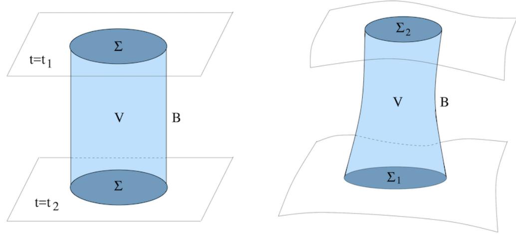
Figure 29. Charge conservation in flat spacetime (on the left) and in curved spacetime (on the right).

4.5.5 The Slippery Business of Energy Conservation

In flat space, the existence of an energy-momentum tensor ensures that we can define the conserved quantities, energy and momentum. In curved spacetime, things are significantly more subtle.

To see this, it’s useful to compare the energy-momentum tensor T^µν $T^{\mu \nu }$ with a current $J^{\mu }$ which arises from a global symmetry (such as, for example, the phase rotation of a complex scalar field). In flat space, both obey current conservation

$${\partial }_{\mu }{J}^{\mu }=0\mathrm{and}{\partial }_{\mu }{T}^{\mu \nu }=0\text{\hspace{1em}(4.56)}$$

From these, we can construct conserved charge by integrating over a spatial volume Σ

$$Q(\Sigma )={\int }_{\Sigma }{d}^{3}x{J}^0\mathrm{and}{P}^{\mu }(\Sigma )={\int }_{\Sigma }{d}^{3}x{T}^{0\mu }$$

To see that these are indeed conserved, we simply need to integrate over a spacetime volume V , bounded by Σ at past and future times $t_1$ and $t_2$ . We then have

$$0={\int }_V{d}^{4}x{\partial }_{\mu }{J}^{\mu }=\Delta Q(\Sigma )+{\int }_B{d}^{3}x{n}_i{J}^i$$

where $\Delta Q(\Sigma )=[Q(\Sigma )](t_2)-[Q(\Sigma )](t_1)$ and $n^i$ is the outward-pointing normal to $B,$ the timelike boundary of $V$ , as shown in the left-hand figure. Provided that no current flows out of the region, meaning $J_i=0$ when evaluated on $B,$ , we have $\Delta Q(\Sigma )=0$ . (Often, we take $\Sigma ={\mathbf{R}}^3$ so that $B={\mathbf{S}}_{\infty }^2\times I$ with I an interval, and we only have to require that there are no currents at infinity.) This is the statement of charge conservation.

In Minkowski space, this same argument works just as well for $P^{\mu }(\Sigma )$ , meaning that we are able to assign conserved energy and momentum to fields in some region, providing that no currents leak out through the boundary.

Let’s now contrast this to the situation in curved spacetime. The conservation laws (4.56) are replaced by their covariant versions

$${\nabla }_{\mu }{J}^{\mu }=0\mathrm{and}{\nabla }_{\mu }{T}^{\mu \nu }=0$$

We can replay the argument above, now invoking the divergence theorem from Section 3.2.4

$$0={\int }_V{d}^{4}x\sqrt{-g}{\nabla }_{\mu }{J}^{\mu }={\int }_{\partial V}{d}^{3}x\sqrt{|\gamma |}{n}_{\mu }{J}^{\mu }$$

with ${\gamma }_{ij}$ the pull-back of the metric to ∂V and $n^{\mu }$ the normal vector. We consider a spacetime volume V with boundary

$$\partial V={\Sigma }_1\cup {\Sigma }_2\cup B$$

Here ${\Sigma }_1$ and ${\Sigma }_2$ are past and future spacelike boundaries, while B is the timelike boundary as shown in the right-hand figure. If we again insist that no current flows out of the region by requiring that $J^{\mu }{n}_{\mu }=0$ when evaluated on B, then the expression above becomes

$$Q({\Sigma }_2)=Q({\Sigma }_1)$$

where the charge $Q(\Sigma )$ evaluated on a spacelike hypersurface Σ is defined by

$$Q(\Sigma )={\int }_{\Sigma }{d}^{3}x\sqrt{\gamma }{n}_{\mu }{J}^{\mu }$$

This means that, for a vector field, covariant conservation is the same thing as actual conservation. The story above is a repeat of the one we told using differential forms in Section 3.2.5.

Now let’s try to tell a similar story for the energy-momentum tensor. In analogy to the derivation above, it’s clear that we should try to manipulate the integral

$$0={\int }_V{d}^{4}x\sqrt{-g}{\nabla }_{\mu }{T}^{\mu \nu }$$

The problem is that we don’t have a divergence theorem for integrals of this kind because of the hanging ν index on the energy momentum tensor. The key to deriving the divergence theorem for $J^{\mu }$ was the expression

$${\nabla }_{\mu }{J}^{\mu }={\partial }_{\mu }{J}^{\mu }+{\Gamma }_{\mu \rho }^{\mu }{J}^{\rho }=\frac{1}{\sqrt{-g}}{\partial }_{\mu }\left(\sqrt{-g}{J}^{\mu }\right)$$

This allows us to turn a covariant derivative into a normal derivative which gives a boundary term in the integral. However, the same expression for the energy-momentum tensor reads

$${\nabla }_{\mu }{T}^{\mu \nu }={\partial }_{\mu }{T}^{\mu \nu }+{\Gamma }_{\mu \rho }^{\mu }{T}^{\rho \nu }+{\Gamma }_{\mu \rho }^{\nu }{T}^{\mu \rho }=\frac{1}{\sqrt{-g}}{\partial }_{\mu }\left(\sqrt{-g}{T}^{\mu \nu }\right)+{\Gamma }_{\mu \rho }^{\nu }{T}^{\mu \rho }$$

That extra term involving the Christoffel symbol stops us converting the integral of ${\nabla }_{\mu }{T}^{\mu \nu }$ into a boundary term. Indeed, we can rewrite ${\nabla }_{\mu }{T}^{\mu \nu }=0$ as

$${\partial }_{\mu }\left(\sqrt{-g}{T}^{\mu \nu }\right)=-\sqrt{-g}{\Gamma }_{\mu \rho }^{\nu }{T}^{\mu \rho }\text{\hspace{1em}(4.57)}$$

then the right-hand side looks like a driving force which destroys conservation of energy and momentum. We learn that, for a higher tensor like $T^{\mu \nu }$ , covariant conservation is not the same thing as actual conservation!

Conserved Energy from a Killing Vector

We can make progress by introducing one further ingredient. If our spacetime has a Killing vector field K, we can construct a current from the energy-momentum tensor by writing

$$J_T^{\nu }=-K_{\mu }{T}^{\mu \nu }$$

Taking the covariant divergence of the current gives

$$-{\nabla }_{\nu }{J}_T^{\nu }=({\nabla }_{\nu }{K}_{\mu })T^{\mu \nu }+K_{\mu }{\nabla }_{\nu }{T}^{\mu \nu }=0$$

where the first term vanishes by virtue of the Killing equation, with $T^{\mu \nu }$ imprinting its symmetric indices on ${\nabla }_{\nu }{K}_{\mu }$ , and the second term vanishes by (4.50).

Now we’re in business. We can construct conserved charges from the current $J_T^{\mu }$ as explained above,

$$Q_T(\Sigma )={\int }_{\Sigma }{d}^{3}x\sqrt{\gamma }{n}_{\mu }{J}_T^{\mu }$$

The interpretation of these charges depends on the properties of the Killing vector. If $K^{\mu }$ is everywhere timelike, meaning $g_{\mu \nu }{K}^{\mu }{K}^{\nu }<0$ at all points, then the charge can be identified with the energy of the matter

$$E=Q_T(\Sigma )$$

If the Killing vector is everywhere spacelike, meaning $g_{\mu \nu }{K}^{\mu }{K}^{\nu }>0$ at all points, then the charge can be identified with the momentum of the matter.

Conserved Energy Without a Killing Vector?

There are situations where spacetime does not have a Killing vector yet, intuitively, we would still like to associate something analogous to energy. This is where things start to get subtle.

A simple situation where this arises is two orbiting stars. It turns out that the resulting spacetime does not admit a timelike Killing vector. As we will describe in some detail in Section 5.3, as the stars orbit they emit gravitational waves, losing energy, which causes them to slowly spiral towards each other. This fits nicely with the lack of a timelike Killing vector, since we wouldn’t expect to define a conserved energy for the stars.

However, it certainly feels like we should be able to define a conserved energy for the total system which, in this case, means stars together with the gravitational waves. In particular, we would like to quantify the amount of energy lost by the stars and carried away by the gravitational waves. But this requires us to define something new, namely the energy density in the gravitational field. And this is where the trouble starts!

There’s an obvious way to proceed, one that starts by returning to our original definition of the energy-momentum tensor (4.46)

$$T_{\mu \nu }=-\frac{2}{\sqrt{-g}}\frac{\delta S_M}{\delta g^{\mu \nu }}$$

A naive guess would be to include the action for both matter and gravity in this definition, giving an energy momentum tensor which includes both matter and gravity

$$T_{\mu \nu }^{\mathrm{total}}=-\frac{2}{\sqrt{-g}}\left(\frac{1}{16\pi G_N}\frac{\delta S_{EH}}{\delta g^{\mu \nu }}+\frac{\delta S_M}{\delta g^{\mu \nu }}\right)$$

But this gives

$$T_{\mu \nu }^{\mathrm{total}}=-\frac{1}{8\pi G_N}{G}_{\mu \nu }+T_{\mu \nu }=0$$

which vanishes by the Einstein field equations. The idea that the total energy of the universe vanishes, with negative gravitational energy cancelling the positive energy from matter sounds like it might be something important. It turns out to be very good for selling pseudo-scientific books designed to make the world think you’re having deep thoughts. It’s not, however, particularly good for anything to do with physics. For example, it’s not as if electrons and positrons are suddenly materialising everywhere in space, their mass energy cancelled by the gravitational energy. That’s not the way the universe works. Instead the right way to think about this equation is to simply appreciate that energy in general relativity is subtle.

Clearly, we should try to do better to understand the energy carried in the gravitational field. Unfortunately, it turns out that doing better is challenging. There are compelling arguments that show there is no tensor that can be thought of as the local energy density of the gravitational field. Roughly speaking, these arguments start from the observation that the energy in the Newtonian gravitational field is proportional to (∇Φ)². We should therefore expect that the relativistic version of energy density is proportional to the first derivative of the metric. Yet the equivalence principle tells us that we can always find coordinates – those experienced by a freely falling observer – which ensure that the first derivative of the metric vanish at any given point. But a tensor that vanishes in one coordinate system also vanishes in another.

We’ll confront these issues again in Section 5.3 when we try to answer the question of how much energy is emitted in gravitational waves by a binary star system. We’ll see there that, for this case, there are simplifications that mean we can converge on a sensible answer.

4.5.6 Spinors

In flat space, fermions transform in the spinor representation of the $SO(1,3)$ Lorentz group. Recall from the lectures on Quantum Field Theory that we first introduce gamma matrices obeying the Clifford algebra

$$\{{\gamma }_a,{\gamma }_b\}=2{\eta }_{ab}\text{\hspace{1em}(4.58)}$$

Notice that we’ve put indices $a,b=0,1,2,3$ on the gamma matrices, rather than the more familiar $\mu ,\nu .$ This is deliberate. In $d=3+1$ dimensions, each of the ${\gamma }_a$ is $\mathrm{a}4\times 4$ matrix.

We can use these gamma matrices to construct generators of the Lorentz group,

$$S_{ab}=\frac{1}{4}[{\gamma }_a,{\gamma }_b]$$

These define the spinor representation of the Lorentz group. We write a Lorentz transformation Λ as

$$\Lambda =\exp \left(\frac{1}{2}{\lambda }^{ab}{M}_{ab}\right)$$

with $M_{ab}$ the usual Lorentz generators (defined, for example, in (4.30)) and ${\lambda }^{ab}$ a choice of 6 numbers that specify the particular Lorentz transformation. Then the corresponding transformation in the spinor representation is given by

$$S[\Lambda ]=\exp \left(\frac{1}{2}{\lambda }^{ab}{S}_{ab}\right)$$

A Dirac spinor field ${\psi }_{\alpha }(x)$ is then a 4-component complex vector that, under a Lorentz transformation, changes as

$$\psi (x)\to S[\Lambda ]\psi ({\Lambda }^{-1}x)\text{\hspace{1em}(4.59)}$$

In Minkowski space, the action for the spinor is

$$S_{\mathrm{Dirac}}=\int d^{4}xi(\bar{\psi }{\gamma }^a{\partial }_a\psi +m\bar{\psi }\psi )$$

with $\bar{\psi }={\psi }^{†}{\gamma }^0$ . The magic of gamma matrices ensures that this action is invariant under Lorentz transformations, despite having just a single derivative. Our task in this section is to generalise this action to curved spacetime.

We can already see some obstacles. The gamma matrices (4.58) are defined in Minkowski space and it’s not clear that they would retain their magic if generalised to curved space. Furthermore, what should we do with the derivative? We might suspect that it gets replaced by a covariant derivative, but what connection do we choose?

To answer these questions, we will need to invoke the vierbeins and connection oneform that we met in Section 3.4.2. Recall that the vierbeins ${\hat{e}}_a=e_a^{\mu }{\partial }_{\mu }$ are a collection of 4 vector fields, that allow us “diagonalise” the metric. We define $e^a{}_{\mu }$ to be the inverse of ${e_a}^{\mu }$ , meaning it satisfies $e^a{}_{\mu }{e}_b{}^{\mu }={\delta }_b^a$ and $e^a{}_{\mu }{e}_a{}^{\nu }={\delta }_{\mu }^{\nu }$ . The metric can then be written

$$g_{\mu \nu }=e_{\mu }^a{e}_{\nu }^b{\eta }_{ab}$$

These formulae are really telling us that we should raise/lower the $\mu ,\nu$ indices using the metric $g_{\mu \nu }$ but raise/lower the $a,b$ indices using the Minkowski metric ${\eta }_{ab}$

The formalism of vierbeins allowed us to introduce the idea of a local Lorentz transformation $\Lambda (x)$ , defined in (3.43), which acts on the vierbeins as

$$e_a^{\nu }\to {\tilde{e}}_a^{\nu }=e_b^{\nu }({\Lambda }^{-1}{)}_a^b\mathrm{with}{\Lambda }_a^c{\Lambda }_b^d{\eta }_{cd}={\eta }_{ab}$$

This local Lorentz transformation can now be promoted to act on a spinor field as (4.59), again with S[Λ] depending on the coordinate x.

We want our action to be invariant under these local Lorentz transformations. In particular, we might expect to run into difficulties with the derivative which, after a Lorentz transformation, now hits $\Lambda (x)$ as well as $\psi (x)$ . But this is exactly the kind of problem that we’ve met before when writing down actions for gauge theories, and we know very well how to solve it: we simply need to include a connection in the action that transforms accordingly. To this end, we construct the covariant derivative acting on a spinor field

$${\nabla }_{\mu }\psi ={\partial }_{\mu }\psi +\frac{1}{2}{\omega }_{\mu }^{ab}{S}_{ab}\psi$$

with ${\omega }_{\mu }^{ab}$ the appropriate connection. But what is it?

The right choice is the connection one-form, also known as the spin connection, that we met in Section 3.4.2. From (3.44) and (3.47), we have

$$({\omega }_b^a{)}_{\mu }={\Gamma }_{cb}^a{e}_{\mu }^c=e_{\rho }^a{\nabla }_{\mu }{e}_b^{\rho }$$

This does the trick because of its inhomogeneous transformation (3.45)

$$({\omega }_b^a{)}_{\mu }\to {\Lambda }_c^a({\omega }_d^c{)}_{\mu }({\Lambda }^{-1}{)}_b^d+{\Lambda }_c^a({\partial }_{\mu }{\Lambda }^{-1}{)}_b^c$$

This cancels the contribution from the derivative in the same way as the covariant derivative in a non-Abelian gauge theory. The generalisation of the Dirac action to curved space is then simply

$$S_{\mathrm{Dirac}}=\int d^{4}x\sqrt{-g}i\left(\bar{\psi }{\gamma }^a{e}_a^{\mu }{\nabla }_{\mu }\psi +m\bar{\psi }\psi \right)$$

There are a number of reasons to be interested in coupling fermions to gravity. First, and most obviously, both are constituents of our universe and its important to understand how they fit together. Second, they are important for more formal aspects of mathematical physics: they are the key component in Witten’s simple proof of the positive mass theorem, and there are reasons to suspect that the quantisation of gravity ultimately requires supersymmetry at a high energy scale.

However, there is one thing that you probably shouldn’t do with them, which is put them on the right-hand side of the Einstein equation and solve them. This is because fermions are quantum fields and do not have a macroscopic, classical analog.

Of course, all fields are, at heart, quantum. But for bosonic fields, it makes sense to think of them classically where they can be viewed as quantum fields with high occupation number. This is familiar in electromagnetism, where the classical electric and magnetic field can be thought of containing many photons. This means that it makes sense to find spacetimes which solve the Einstein equations $G_{\mu \nu }=8\pi G{T}_{\mu \nu }$ where the curvature is supported by a profile for scalar fields on the right-hand-side.

In contrast, there is no classical limit of fermionic fields. This is because the Pauli exclusion principle prohibits a large occupation number. If you therefore attempt to find a spacetime supported by a fermionic $T_{\mu \nu },$ you are really looking for a gravitational solution sourced by precisely one quantum excitation. Given the feebleness of gravity on the microscopic scale, this is unlikely to be interesting.

This is not to say that fermions don’t affect gravity. Important examples for gravitating fermionic systems include white dwarfs and neutron stars. But in each of these cases there is a separation of scales where one can first neglect gravity and find an effective equation of state for the fermions, and subsequently understand how this backreacts on spacetime. If you want to understand the spacetime directly from the Dirac equation than you have a complicated many-body problem on your hands.

4.5.7 Energy Conditions

If we know the kind of matter that fills spacetime, then we can just go ahead and solve the Einstein equations. However, we will often want to make more general statements about the allowed properties of spacetime without reference to any specific matter content. In this case, it is useful to place certain restrictions on the kinds of energymomentum tensor that we consider physical.

These restrictions, known as energy conditions, capture the rough idea that energy should be positive. A number of classic results in general relativity, such as the singularity theorems, rely on these energy conditions as assumptions.

There are a bewildering number of these energy conditions. Moreover, it is not difficult to find examples of matter which violate most of them! We now describe a number of the most important energy conditions, together with their limitations.

• Weak Energy Condition: This states that, for any timelike vector field X,

$$T_{\mu \nu }{X}^{\mu }{X}^{\nu }\ge 0\mathrm{forall}X\mathrm{with}{X}_{\mu }{X}^{\mu }<0$$

The idea is that this quantity is the energy seen by an observer moving along the timelike integral curves of X, and this should be non-negative. A timelike curve can get arbitrarily close to a null curve so, by continuity, the weak energy condition can be extended to timelike and null curves

$$T_{\mu \nu }{X}^{\mu }{X}^{\nu }\ge 0\mathrm{forall}X\mathrm{with}{X}_{\mu }{X}^{\mu }\le 0\text{\hspace{1em}(4.60)}$$

To get a feel for this requirement, let’s first impose it on the energy-momentum tensor for a perfect fluid (4.53). We will consider timelike vectors X normalised

to $X\cdot X=-1$ . We then have

$$T_{\mu \nu }{X}^{\mu }{X}^{\nu }=(\rho +P)(u\cdot X{)}^2-P\ge 0$$

We work in the rest frame of the fluid, so $u^{\mu }=\left(1,0,0,0\right)$ and consider constant timelike vector fields, $X^{\mu }=(\cosh \phi ,$ , sinh $\phi ,0,0)$ . These describe the worldlines of observers boosted with rapidity $\phi$ with respect to the fluid. The weak energy condition then gives us

$$(\rho +P){\cosh }^2\phi -P\ge 0\Rightarrow \{\begin{array}{l}\rho \ge 0\text{when}\phi =0\\ P\ge -\rho \text{as}\phi \to \infty \end{array}$$

The first condition $\rho \ge 0$ is what we expect from the weak energy condition: it ensures that the energy density is positive. The second condition $P\ge -\rho$ says that negative pressure is acceptable, just as long as it’s not too negative.

There are, however, situations in which negative energy density makes physical sense. Indeed, we’ve met one already: if we view the cosmological constant as part of the energy momentum tensor, as in (4.48), then any $\Lambda <0$ violates the weak energy condition. Viewed this way, anti-de Sitter spacetime violates the weak energy condition.

We can also look at how this condition fares for scalar fields. From the energymomentum tensor (4.51), we have

$$(X^{\mu }{\partial }_{\mu }\varphi {)}^2+\frac{1}{2}{\partial }_{\mu }\varphi {\partial }^{\mu }\varphi +V(\varphi )\ge 0\text{\hspace{1em}(4.61)}$$

The first term is positive, but the second term can have either sign. In fact, it turns out that the first and second term combined are always positive. To see this, define the vector $Y$ orthogonal to $X$

$$Y_{\mu }={\partial }_{\mu }\varphi +X_{\mu }(X^{\nu }{\partial }_{\nu }\varphi )$$

This satisfies $X_{\mu }{Y}^{\mu }=0$ : it is the projection of ${\partial }_{\mu }\varphi$ onto directions orthogonal to $X$ . Because $X$ is timelike, Y must be spacelike (or null) and so obeys $Y_{\mu }{Y}^{\mu }\ge 0$ The weak energy condition (4.61) can be rewritten as

$$\frac{1}{2}(X^{\mu }{\partial }_{\mu }\varphi {)}^2+\frac{1}{2}{Y}_{\mu }{Y}^{\mu }+V(\varphi )\ge 0$$

Now the first two terms are positive. We see that the weak energy condition is satisfied provided that $V(\varphi )\ge 0$ . However, it is violated in any classical theory with $V(\varphi )\le 0$ and there’s no reason to forbid such negative potentials for a scalar field.

• Strong Energy Condition: There is a different, less immediately intuitive, energy condition. This is the requirement that, for any timelike vector field X,

$$R_{\mu \nu }{X}^{\mu }{X}^{\nu }\ge 0$$

This is the strong energy condition. It is poorly named. The strong energy condition is neither stronger nor weaker than the weak energy condition: it is simply different. It turns out that the strong energy condition ensures that timelike geodesics converge, which can be viewed as the statement that gravity is attractive. (This connection is made using something called the Raychaudhuri equation.)

Using the form of the Einstein equations (4.49), the strong energy condition requires

$$\left(T_{\mu \nu }-\frac{1}{2}T{g}_{\mu \nu }\right)X^{\mu }{X}^{\nu }\ge 0$$

for all timelike vector fields X. As before, continuity ensures that we can extend this to timelike and null vector fields, $X\cdot X\le 0$

If we take $X\cdot X=-1$ then, applied to a perfect fluid (4.53), the strong energy condition requires

$$(\rho +P)(u\cdot X{)}^2-P+\frac{1}{2}(3P-\rho )\ge 0$$

As before, we consider the fluid in its rest frame with $u^{\mu }=\left(1,0,0,0\right)$ and look at this condition for boosted observers with $X^{\mu }=(\cosh {\phi }_{;}$ , sinh $\phi ,0,0)$ . We have

$$(\rho +P){\cosh }^2\phi +\frac{1}{2}(P-\rho )\ge 0\Rightarrow \{\begin{array}{ll}P\ge -\rho /3& \phi =0\\ P\ge -\rho & \phi \to \infty \end{array}$$

Once again, it is not difficult to find situations where the strong energy condition is violated. Most strikingly, a cosmological constant $\Lambda >0$ is not compatible with the strong energy condition. In fact, we may have suspected this because neighbouring, timelike geodesics in de Sitter space are pulled apart by the expansion of space. In fact, the strong energy condition forbids any FRW universe with $\ddot{a}>0$ but there are at least two periods when our own universe underwent accelerated expansion: during inflation, and now.

Finally, it’s not hard to show that any classical scalar field with a positive potential energy will violate the strong energy condition.

• Null Energy Condition: The null energy condition

$$T_{\mu \nu }{X}^{\mu }{X}^{\nu }\ge 0\text{ for all }X\text{ with }X\cdot X=0$$

This is implied by both weak and strong energy conditions, but the converse is not true: the null energy condition is strictly weaker than both the weak and strong conditions. This, of course, means that it is less powerful if we wield it to prove various statements. However, the null energy condition has the advantage that it is satisfied by any sensible classical field theory and any perfect fluid that obeys $\rho +P\ge 0$

• Dominant Energy Condition: There is also an energy condition which is stronger than the weak condition. For any future-directed timelike vector X, we can define the current

$$J^{\mu }=-T^{\mu \nu }{X}_{\nu }\text{\hspace{1em}(4.62)}$$

This is energy density current as seen by an observer following the lines of X. The dominant energy condition requires that, in addition to the weak energy condition (4.60), the current is either timelike or null, so

$$J_{\mu }{J}^{\mu }\le 0$$

This is the reasonable statement that energy doesn’t flow faster than light.

One can check that the extra condition (4.62) is satisfied for a scalar field. For a perfect fluid we have

$$J^{\mu }=-(\rho +P)(u\cdot X)u^{\mu }-P{X}^{\mu }$$

It’s simple to check that the requirement $J_{\mu }{J}^{\mu }\le 0$ is simply ${\rho }^2\ge P^2$

The validity of the various energy conditions becomes murkier still in the quantum world. We can consider quantum matter coupled to a classical yet dynamical spacetime through the equation

$$G_{\mu \nu }+\Lambda g_{\mu \nu }=8\pi G⟨T_{\mu \nu }⟩$$

where $T_{\mu \nu }$ is the expectation value of the energy-momentum tensor. Each of the energy conditions listed above is violated by fairly standard quantum field theories.

There is, however, a somewhat weaker statement that holds true in general. This is the averaged null energy condition. It can be proven that, along an infinite, achronal null geodesic, any reasonable quantum field theory obeys

$${\int }_{-\infty }^{+\infty }d\lambda ⟨T_{\mu \nu }⟩X^{\mu }{X}^{\nu }\ge 0$$

Here λ is an affine parameter along the null geodesic and the vector $X^{\mu }$ points along the geodesic and is normalised to $X^{\mu }{\partial }_{\mu }\lambda =1$ . Here the word “achronal” means that no two points on the geodesic can be connected by a timelike curve. (As a counterexample, consider an infinite null ray on $M=\mathbf{R}\times {\mathbf{S}}^1$ which continually orbits the spatial circle. This geodesic is not achronal and the averaged null energy condition is not, in general, obeyed along this geodesic.)

来源与版本

正文：英文 · OCR 机器稿 · 待校对

核对状态：OCR 机器稿 · 待校对

原书 PDF

来源版本：michaelmas-2019-source-20260923

来源 PDF SHA-256：3ba65dc61f22a69c7d5fdf3e8e1f641efbfa6cf49a44b3dcb0fd5367ba9fcf1c

OCR 来源 SHA-256：988fe63d50521107cf7e476ccf517496c8ba2ca839cea1e6e9e5e0bcf9ce0f79

OCR 产物 SHA-256：998ccf7adad8e7d060b8e45747c12df3f869b8c074718c17f53b02141136837e