3.2 Connections and Curvature

We’ve already met one version of differentiation in these lectures. A vector field X is, at heart, a differential operator and provides a way to differentiate a function $f$ . We write this simply as $X(f)$

As we saw previously, differentiating higher tensor fields is a little more tricky because it requires us to subtract tensor fields at different points. Yet tensors evaluated at different points live in different vector spaces, and it only makes sense to subtract these objects if we can first find a way to map one vector space into the other. In Section 2.2.4, we used the flow generated by X as a way to perform this mapping, resulting in the idea of the Lie derivative ${\mathcal{L}}_X$

There is, however, a different way to take derivatives, one which ultimately will prove more useful. The derivative is again associated to a vector field X. However, this time we introduce a different object, known as a connection to map the vector spaces at one point to the vector spaces at another. The result is an object, distinct from the Lie derivative, called the covariant derivative.

3.2.1 The Covariant Derivative

A connection is a map $\nabla :\mathfrak{X}(M)\times \mathfrak{X}(M)\to \mathfrak{X}(M)$ . We usually write this as $\nabla (X,Y)=$ ${\nabla }_{X}Y$ and the object ${\nabla }_X$ is called the covariant derivative. It satisfies the following properties for all vector fields X, Y and Z,

$$\bullet {\nabla }_X(Y+Z)={\nabla }_{X}Y+{\nabla }_{X}Z$$

${\nabla }_{(fX+gY)}Z=f{\nabla }_{X}Z+g{\nabla }_{Y}Z$ for all functions $f,g$

${\nabla }_X(fY)=f{\nabla }_{X}Y+({\nabla }_{X}f)Y$ where we define ${\nabla }_{X}f=X(f)$

The covariant derivative endows the manifold with more structure. To elucidate this, we can evaluate the connection in a basis $\{e_{\mu }\}$ of $\mathfrak{X}(M)$ . We can always express this as

$${\nabla }_{e_{\rho }}{e}_{\nu }={\Gamma }_{\rho \nu }^{\mu }{e}_{\mu }\text{\hspace{1em}(3.8)}$$

with ${\Gamma }_{\rho \nu }^{\mu }$ the components of the connection. It is no coincidence that these are denoted by the same greek letter that we used for the Christoffel symbols in Section 1. However, for now, you should not conflate the two; we’ll see the relationship between them in Section 3.2.3.

The name “connection” suggests that ∇, or its components ${\Gamma }_{\nu \rho }^{\mu },$ connect things. Indeed they do. We will show in Section 3.3 that the connection provides a map from the tangent space $T_p(M)$ to the tangent space at any other point $T_q(M)$ . This is what allows the connection to act as a derivative.

We will use the notation

$${\nabla }_{\mu }={\nabla }_{e_{\mu }}$$

This makes the covariant derivative ${\nabla }_{\mu }$ look similar to a partial derivative. Using the properties of the connection, we can write a general covariant derivative of a vector field as

$$\begin{array}{rl}& {\nabla }_{X}Y={\nabla }_X(Y^{\mu }{e}_{\mu })\\ & =X(Y^{\mu })e_{\mu }+Y^{\mu }{\nabla }_X{e}_{\mu }\\ & =X^{\nu }{e}_{\nu }(Y^{\mu })e_{\mu }+X^{\nu }{Y}^{\mu }{\nabla }_{\nu }{e}_{\mu }\\ & =X^{\nu }\left(e_{\nu }(Y^{\mu })+{\Gamma }_{\nu \rho }^{\mu }{Y}^{\rho }\right)e_{\mu }\end{array}$$

The fact that we can strip of the overall factor of $X^{\nu }$ means that it makes sense to write the components of the covariant derivative as

$${\nabla }_{\nu }Y=(e_{\nu }(Y^{\mu })+{\Gamma }_{\nu \rho }^{\mu }{Y}^{\rho })e_{\mu }$$

Or, in components,

$$({\nabla }_{\nu }Y{)}^{\mu }=e_{\nu }(Y^{\mu })+{\Gamma }_{\nu \rho }^{\mu }{Y}^{\rho }\text{\hspace{1em}(3.9)}$$

Note that the covariant derivative coincides with the Lie derivative on functions, ${\nabla }_{X}f=$ ${\mathcal{L}}_{X}f=X(f)$ . It also coincides with the old-fashioned partial derivative: ${\nabla }_{\mu }f={\partial }_{\mu }f$ However, its action on vector fields differs. In particular, the Lie derivative ${\mathcal{L}}_{X}Y=$ [X, Y] depends on both X and the first derivative of X while, as we have seen above, the covariant derivative depends only on X. This is the property that allows us to write ${\nabla }_X=X^{\nu }{\nabla }_{\nu }$ and think of ${\nabla }_{\mu }$ as an operator in its own right. In contrast, there is no way to write ${}^{\mathfrak{a}}{\mathcal{L}}_X=X^{\mu }{\mathcal{L}}_{\mu }{}^3$ . While the Lie derivative has its uses, the ability to define ${\nabla }_{\mu }$ means that this is best viewed as the natural generalisation of the partial derivative to curved space.

Differentiation as Punctuation

In a coordinate basis, in which $e_{\mu }={\partial }_{\mu }$ , the covariant derivative (3.9) becomes

$$({\nabla }_{\nu }Y{)}^{\mu }={\partial }_{\nu }{Y}^{\mu }+{\Gamma }_{\nu \rho }^{\mu }{Y}^{\rho }\text{\hspace{1em}(3.10)}$$

We will differentiate often. To save ink, we use the sloppy, and sometimes confusing, notation

$$({\nabla }_{\nu }Y{)}^{\mu }={\nabla }_{\nu }{Y}^{\mu }$$

This means, in particular, that ${\nabla }_{\nu }{Y}^{\mu }$ is the ${\mu }^{\mathrm{th}}$ component of ${\nabla }_{\nu }Y$ , rather than the differentiation of the function $Y^{\mu }$

Covariant differentiation is sometimes denoted using a semi-colon

$${\nabla }_{\nu }{Y}^{\mu }=Y_{;\nu }^{\mu }$$

In this convention, the partial derivative is denoted using a mere comma, ${\partial }_{\mu }{Y}^{\nu }=Y^{\nu }{}_{,\mu }$ The expression (3.10) then reads

$$Y_{;\nu }^{\mu }=Y_{,\nu }^{\mu }+{\Gamma }_{\nu \rho }^{\mu }{Y}^{\rho }$$

I’m proud to say that we won’t adopt the “semi-colon = differentiation” notation in these lectures. Because it’s stupid.

The Connection is Not a Tensor

The ${\Gamma }^{\mu }{}_{\rho \nu }$ defining the connection are not components of a tensor. We can see this immediately from the definition $\nabla (X,fY)={\nabla }_X(fY)=f{\nabla }_{X}Y+(X(f))Y$ . This is not linear in the second argument, which is one of the requirements of a tensor.

To illustrate this, we can ask what the connection looks like in a different basis,

$${\tilde{e}}_{\nu }=A_{\nu }^{\mu }{e}_{\mu }\text{\hspace{1em}(3.11)}$$

for some invertible matrix A. If $e_{\mu }$ and ${\tilde{e}}_{\mu }$ are both coordinate bases, then

$$A_{\nu }^{\mu }=\frac{\partial x^{\mu }}{\partial {\tilde{x}}^{\nu }}$$

We know from (2.23) that the components of a (1, 2) tensor transform as

$${\tilde{T}}_{\nu \rho }^{\mu }=(A^{-1}{)}_{\tau }^{\mu }{A}_{\nu }^{\lambda }{A}_{\rho }^{\sigma }{T}_{\lambda \sigma }^{\tau }\text{\hspace{1em}(3.12)}$$

We can now compare this to the transformation of the connection components ${\Gamma }_{\rho \nu }^{\mu }$ . In the basis ${\tilde{e}}_{\mu }$ , we have

$${\nabla }_{{\tilde{e}}_{\rho }}{\tilde{e}}_{\nu }={\tilde{\Gamma }}_{\rho \nu }^{\mu }{\tilde{e}}_{\mu }$$

Substituting in the transformation (3.11), we have

$${\tilde{\Gamma }}_{\rho \nu }^{\mu }{\tilde{e}}_{\mu }={\nabla }_{(A_{\rho }^{\sigma }{e}_{\sigma })}(A_{\nu }^{\lambda }{e}_{\lambda })=A_{\rho }^{\sigma }{\nabla }_{e_{\sigma }}(A_{\nu }^{\lambda }{e}_{\lambda })=A_{\rho }^{\sigma }{A}_{\nu }^{\lambda }{\Gamma }_{\sigma \lambda }^{\tau }{e}_{\tau }+A_{\rho }^{\sigma }{e}_{\lambda }{\partial }_{\sigma }{A}_{\nu }^{\lambda }$$

We can write this as

$$\begin{array}{rl}& {\tilde{\Gamma }}_{\rho \nu }^{\mu }{\tilde{e}}_{\mu }=(A_{\rho }^{\sigma }{A}_{\nu }^{\lambda }{\Gamma }_{\sigma \lambda }^{\tau }+A_{\rho }^{\sigma }{\partial }_{\sigma }{A}_{\nu }^{\tau })e_{\tau }\\ & =(A_{\rho }^{\sigma }{A}_{\nu }^{\lambda }{\Gamma }_{\sigma \lambda }^{\tau }+A_{\rho }^{\sigma }{\partial }_{\sigma }{A}_{\nu }^{\tau })(A^{-1}{)}_{\tau }^{\mu }{\tilde{e}}_{\mu }\end{array}$$

Stripping of the basis vectors ${\tilde{e}}_{\mu }$ , we see that the components of the connection transform as

$${\tilde{\Gamma }}_{\rho \nu }^{\mu }=(A^{-1}{)}_{\tau }^{\mu }{A}_{\rho }^{\sigma }{A}_{\nu }^{\lambda }{\Gamma }_{\sigma \lambda }^{\tau }+(A^{-1}{)}_{\tau }^{\mu }{A}_{\rho }^{\sigma }{\partial }_{\sigma }{A}_{\nu }^{\tau }\text{\hspace{1em}(3.13)}$$

The first term coincides with the transformation of a tensor (3.12). But the second term, which is independent of Γ, but instead depends on $\partial A$ , is novel. This is the characteristic transformation property of a connection.

Differentiating Other Tensors

We can use the Leibniz property of the covariant derivative to extend its action to any tensor field. It’s best to illustrate this with an example.

Consider a one-form ω. If we differentiate $\omega ,$ we will get another one-form ${\nabla }_X\omega$ which, like any one-form, is defined by its action on vector fields $Y\in \mathfrak{X}(M)$ To construct this, we will insist that the connection obeys Leibniz in the modified sense that

$${\nabla }_X(\omega (Y))=({\nabla }_X\omega )(Y)+\omega ({\nabla }_{X}Y)$$

But $\omega (Y)$ is simply a function, which means that we can also write this as

$${\nabla }_X(\omega (Y))=X(\omega (Y))$$

Putting these together gives

$$({\nabla }_X\omega )(Y)=X(\omega (Y))-\omega ({\nabla }_{X}Y)$$

In coordinates, we have

$$\begin{array}{rl}& X^{\mu }({\nabla }_{\mu }\omega {)}_{\nu }{Y}^{\nu }=X^{\mu }{\partial }_{\mu }({\omega }_{\nu }{Y}^{\nu })-{\omega }_{\nu }{X}^{\mu }({\partial }_{\mu }{Y}^{\nu }+{\Gamma }_{\mu \rho }^{\nu }{Y}^{\rho })\\ & =X^{\mu }({\partial }_{\mu }{\omega }_{\rho }-{\Gamma }_{\mu \rho }^{\nu }{\omega }_{\nu })Y^{\rho }\end{array}$$

where, crucially, the $\partial Y$ terms cancel in going from the first to the second line. This means that the overall result is linear in Y and we may define ${\nabla }_X\omega$ without reference to the vector field $Y$ on which is acts. In components, we have

$$({\nabla }_{\mu }\omega {)}_{\rho }={\partial }_{\mu }{\omega }_{\rho }-{\Gamma }_{\mu \rho }^{\nu }{\omega }_{\nu }$$

As for vector fields, we also write this as

$$({\nabla }_{\mu }\omega {)}_{\rho }\equiv {\nabla }_{\mu }{\omega }_{\rho }\equiv {\omega }_{\rho ;\mu }={\omega }_{\rho ,\mu }-{\Gamma }_{\mu \rho }^{\nu }{\omega }_{\nu }$$

This kind of argument can be extended to a general tensor field of rank $(p,q)$ , where the covariant derivative is defined by,

$$\begin{array}{rl}& T_{{\nu }_1\dots {\nu }_q;\rho }^{{\mu }_1\dots {\mu }_p}=T_{{\nu }_1\dots {\nu }_q,\rho }^{{\mu }_1\dots {\mu }_p}+{\Gamma }_{\rho \sigma }^{{\mu }_1}{T}_{{\nu }_1\dots {\nu }_q}^{\sigma {\mu }_2\dots {\mu }_p}+\dots +{\Gamma }_{\rho \sigma }^{{\mu }_p}{T}_{{\nu }_1\dots {\nu }_q}^{{\mu }_1\dots {\mu }_{p-1}\sigma }\\ & -{\Gamma }_{\rho {\nu }_1}^{\sigma }{T}_{\sigma {\nu }_2\dots {\nu }_q}^{{\mu }_1\dots {\mu }_p}-\dots -{\Gamma }_{\rho {\nu }_q}^{\sigma }{T}_{{\nu }_1\dots {\nu }_{q-1}\sigma }^{{\mu }_1\dots {\mu }_p}\end{array}$$

The pattern is clear: for every upper index $\mu$ we get $\mathrm{a}+\Gamma T$ term, while for every lower index we get $\mathrm{a}-\Gamma T$ term.

Now that we can differentiate tensors, we will also need to extend our punctuation notation slightly. If more than two subscripts follow a semi-colon (or, indeed, a comma) then we differentiate respect to both, doing the one on the left first. So, for example, ${X^{\mu }}_{;\nu \rho }={\nabla }_{\rho }{\nabla }_{\nu }{X}^{\mu }$

3.2.2 Torsion and Curvature

Even though the connection is not a tensor, we can use it to construct two tensors. The first is a rank (1, 2) tensor $T$ known as torsion. It is defined to act on $X,Y\in \mathfrak{X}(M)$ and $\omega \in {\Lambda }^1(M)$ by

$$T(\omega ;X,Y)=\omega ({\nabla }_{X}Y-{\nabla }_{Y}X-[X,Y])$$

The other is a rank (1, 3) tensor $R,$ known as curvature. It acts on $X,Y,Z\in \mathfrak{X}(M)$ and $\omega \in {\Lambda }^1(M)$ by

$$R(\omega ;X,Y,Z)=\omega ({\nabla }_X{\nabla }_{Y}Z-{\nabla }_Y{\nabla }_{X}Z-{\nabla }_{[X,Y]}Z)$$

The curvature tensor is also called the Riemann tensor.

Alternatively, we could think of torsion as a map $T:\mathfrak{X}(M)\times \mathfrak{X}(M)\to \mathfrak{X}(M)$ , defined by

$$T(X,Y)={\nabla }_{X}Y-{\nabla }_{Y}X-[X,Y]$$

Similarly, the curvature R can be viewed as a map from $\mathfrak{X}(M)\times \mathfrak{X}(M)$ to a differential operator acting on $\mathfrak{X}(M)$

$$R(X,Y)={\nabla }_X{\nabla }_Y-{\nabla }_Y{\nabla }_X-{\nabla }_{[X,Y]}\text{\hspace{1em}(3.14)}$$

Checking Linearity

To demonstrate that T and R are indeed tensors, we need to show that they are linear in all arguments. Linearity in ω is straightforward. For the others, there are some small calculations to do. For example, we must show that $T(\omega ;fX,Y)=fT(\omega ;X,Y)$ . To see this, we just run through the definitions of the various objects,

$$T(\omega ;fX,Y)=\omega \left({\nabla }_{fX}Y-{\nabla }_Y(fX)-[fX,Y]\right)$$

We then use ${\nabla }_{fX}Y=f{\nabla }_{X}Y$ and ${\nabla }_Y(fX)=f{\nabla }_{Y}X+Y(f)$ X and $[fX,Y]=f[X,Y]-$ $Y(f)X$ . The two $Y(f)X$ terms cancel, leaving us with

$$\begin{array}{c}T(\omega ;fX,Y)=f\omega ({\nabla }_{X}Y-{\nabla }_{Y}X-[X,Y])\\ =fT(\omega ;X,Y)\end{array}$$

Similarly, for the curvature tensor we have

$$\begin{array}{rl}& R(\omega ;fX,Y,Z)=\omega ({\nabla }_{fX}{\nabla }_{Y}Z-{\nabla }_Y{\nabla }_{fX}Z-{\nabla }_{[fX,Y]}Z\\ & =\omega (f{\nabla }_X{\nabla }_{Y}Z-{\nabla }_Y(f{\nabla }_{X}Z)-{\nabla }_{(f[X,Y]-Y(f)X)}Z)\\ & =\omega (f{\nabla }_X{\nabla }_{Y}Z-f{\nabla }_Y{\nabla }_{X}Z-Y(f){\nabla }_{X}Z-{\nabla }_{f[X,Y]}Z+{\nabla }_{Y(f)X}Z)\\ & =\omega (f{\nabla }_X{\nabla }_{Y}Z-f{\nabla }_Y{\nabla }_{X}Z-Y(f){\nabla }_{X}Z-f{\nabla }_{[X,Y]}Z+Y(f){\nabla }_{X}Z)\\ & =f\omega ({\nabla }_X{\nabla }_{Y}Z-{\nabla }_Y{\nabla }_{X}Z-{\nabla }_{[X,Y]}Z)\\ & =fR(\omega ;X,Y,Z)\end{array}$$

Linearity in Y follows from linearity in X. But we still need to check linearity in $Z.$

$$\begin{array}{rl}& R(\omega ;X,Y,fZ)=\omega ({\nabla }_X{\nabla }_Y(fZ)-{\nabla }_Y{\nabla }_X(fZ)-{\nabla }_{[X,Y]}(fZ))\\ & =\omega ({\nabla }_X(f{\nabla }_{Y}Z+Y(f)Z)-{\nabla }_Y(f{\nabla }_{X}Z+X(f)Z)\\ & -f{\nabla }_{[X,Y]}Z-[X,Y](f)Z)\\ & =\omega (f{\nabla }_X{\nabla }_{Y}Z+X(f){\nabla }_{Y}Z+Y(f){\nabla }_{X}Z+X(Y(f))Z\\ & -f{\nabla }_Y{\nabla }_{X}Z-Y(f){\nabla }_{X}Z-X(f){\nabla }_{Y}Z-Y(X(f))Z\\ & -f{\nabla }_{[X,Y]}Z-[X,Y](f)Z)\\ & =fR(\omega ;X,Y,Z)\end{array}$$

Thus, both torsion and curvature define new tensors on our manifold.

Components

We can evaluate these tensors in a coordinate basis $\{e_{\mu }\}=\{{\partial }_{\mu }\}$ , with the dual basis $\{f^{\mu }\}=\{d{x}^{\mu }\}$ . The components of the torsion are

$$\begin{array}{rl}& T_{\mu \nu }^{\rho }=T(f^{\rho };e_{\mu },e_{\nu })\\ & =f^{\rho }({\nabla }_{\mu }{e}_{\nu }-{\nabla }_{\nu }{e}_{\mu }-[e_{\mu },e_{\nu }])\\ & =f^{\rho }({\Gamma }_{\mu \nu }^{\sigma }{e}_{\sigma }-{\Gamma }_{\nu \mu }^{\sigma }{e}_{\sigma })\\ & ={\Gamma }_{\mu \nu }^{\rho }-{\Gamma }_{\nu \mu }^{\rho }\end{array}$$

where we’ve used the fact that, in a coordinate basis, $[e_{\mu },e_{\nu }]=[{\partial }_{\mu },{\partial }_{\nu }]=0$ . We learn that, even though ${\Gamma }_{\mu \nu }^{\rho }$ is not a tensor, the anti-symmetric part ${\Gamma }_{[\mu \nu ]}^{\rho }$ does form a tensor. Clearly the torsion tensor is anti-symmetric in the lower two indices

$$T_{\mu \nu }^{\rho }=-T_{\nu \mu }^{\rho }$$

Connections which are symmetric in the lower indices, so ${\Gamma }_{\mu \nu }^{\rho }={\Gamma }_{\nu \mu }^{\rho }$ have $T^{\rho }{}_{\mu \nu }=0$ Such connections are said to be torsion-free.

The components of the curvature tensor are given by

$$R_{\rho \mu \nu }^{\sigma }=R(f^{\sigma };e_{\mu },e_{\nu },e_{\rho })$$

Note the slightly counterintuitive, but standard ordering of the indices; the indices µ and ν that are associated to covariant derivatives ${\nabla }_{\mu }$ and ${\nabla }_{\nu }$ go at the end. We have

$$\begin{array}{rl}{R}_{\rho \mu \nu }^{\sigma }=f^{\sigma }({\nabla }_{\mu }{\nabla }_{\nu }{e}_{\rho }-{\nabla }_{\nu }{\nabla }_{\mu }{e}_{\rho }-{\nabla }_{[e_{\mu },e_{\nu }]}{e}_{\rho })& \\ & =f^{\sigma }({\nabla }_{\mu }{\nabla }_{\nu }{e}_{\rho }-{\nabla }_{\nu }{\nabla }_{\mu }{e}_{\rho })\\ & =f^{\sigma }({\nabla }_{\mu }({\Gamma }_{\nu \rho }^{\lambda }{e}_{\lambda })-{\nabla }_{\nu }({\Gamma }_{\mu \rho }^{\lambda }{e}_{\lambda }))\\ & =f^{\sigma }(({\partial }_{\mu }{\Gamma }_{\nu \rho }^{\lambda })e_{\lambda }+{\Gamma }_{\nu \rho }^{\lambda }{\Gamma }_{\mu \lambda }^{\tau }{e}_{\tau }-({\partial }_{\nu }{\Gamma }_{\mu \rho }^{\lambda })e_{\lambda }-{\Gamma }_{\mu \rho }^{\lambda }{\Gamma }_{\nu \lambda }^{\tau }{e}_{\tau })\\ & ={\partial }_{\mu }{\Gamma }_{\nu \rho }^{\sigma }-{\partial }_{\nu }{\Gamma }_{\mu \rho }^{\sigma }+{\Gamma }_{\nu \rho }^{\lambda }{\Gamma }_{\mu \lambda }^{\sigma }-{\Gamma }_{\mu \rho }^{\lambda }{\Gamma }_{\nu \lambda }^{\sigma }\end{array}\text{\hspace{1em}(3.15)}$$

Clearly the Riemann tensor is anti-symmetric in its last two indices

$$R_{\rho \mu \nu }^{\sigma }=-R_{\rho \nu \mu }^{\sigma }$$

Equivalently, $R^{\sigma }{}_{\rho \mu \nu }=R^{\sigma }{}_{\rho [\mu \nu ]}$ . There are a number of further identities of the Riemann tensor of this kind. We postpone this discussion to Section 3.4.

The Ricci Identity

There is a closely related calculation in which both the torsion and Riemann tensors appears. We look at the commutator of covariant derivatives acting on vector fields. Written in an orgy of anti-symmetrised notation, this calculation gives

$$\begin{array}{rl}& {\nabla }_{[\mu }{\nabla }_{\nu ]}{Z}^{\sigma }={\partial }_{[\mu }({\nabla }_{\nu ]}{Z}^{\sigma })+{\Gamma }_{[\mu |\lambda |}^{\sigma }{\nabla }_{\nu ]}{Z}^{\lambda }-{\Gamma }_{[\mu \nu ]}^{\rho }{\nabla }_{\rho }{Z}^{\sigma }\\ & ={\partial }_{[\mu }{\partial }_{\nu ]}{Z}^{\sigma }+({\partial }_{[\mu }{\Gamma }_{\nu ]\rho }^{\sigma })Z^{\rho }+({\partial }_{[\mu }{Z}^{\rho }){\Gamma }_{\nu ]\rho }^{\sigma }+{\Gamma }_{[\mu |\lambda |}^{\sigma }{\partial }_{\nu ]}{Z}^{\lambda }\\ & +{\Gamma }_{[\mu |\lambda |}^{\sigma }{\Gamma }_{\nu ]\rho }^{\lambda }{Z}^{\rho }-{\Gamma }_{[\mu \nu ]}^{\rho }{\nabla }_{\rho }{Z}^{\sigma }\end{array}$$

The first term vanishes, while the third and fourth terms cancel against each other. We’re left with

$$2{\nabla }_{[\mu }{\nabla }_{\nu ]}{Z}^{\sigma }=R_{\rho \mu \nu }^{\sigma }{Z}^{\rho }-T_{\mu \nu }^{\rho }{\nabla }_{\rho }{Z}^{\sigma }\text{\hspace{1em}(3.16)}$$

where the torsion tensor is $T^{\rho }{}_{\mu \nu }=2{\Gamma }_{[\mu \nu ]}^{\rho }$ and the Riemann tensor appears as

$$R_{\rho \mu \nu }^{\sigma }=2{\partial }_{[\mu }{\Gamma }_{\nu ]\rho }^{\sigma }+2{\Gamma }_{[\mu |\lambda |}^{\sigma }{\Gamma }_{\nu ]\rho }^{\lambda }$$

which coincides with (3.15). The expression (3.16) is known as the Ricci identity.

3.2.3 The Levi-Civita Connection

So far, our discussion of the connection $\nabla$ has been entirely independent of the metric. However, something nice happens if we have both a connection and a metric. This something nice is called the fundamental theorem of Riemannian geometry. (Happily, it’s also true for Lorentzian geometries.)

Theorem

There exists a unique, torsion free, connection that is compatible with a metric g, in the sense that

$${\nabla }_{X}g=0$$

for all vector fields X.

Proof

We start by showing uniqueness. Suppose that such a connection exists. Then, by Leibniz

$$X(g(Y,Z))={\nabla }_X(g(Y,Z))=({\nabla }_{X}g)(Y,Z)+g({\nabla }_{X}Y,Z)+g(Y,{\nabla }_{X}Z)$$

Since ${\nabla }_{X}g=0$ , this becomes

$$X(g(Y,Z))=g({\nabla }_{X}Y,Z)+g({\nabla }_{X}Z,Y)$$

By cyclic permutation of X, Y and Z, we also have

$$\begin{array}{rl}& Y(g(Z,X))=g({\nabla }_{Y}Z,X)+g({\nabla }_{Y}X,Z)\\ & Z(g(X,Y))=g({\nabla }_{Z}X,Y)+g({\nabla }_{Z}Y,X)\end{array}$$

Since the torsion vanishes, we have

$${\nabla }_{X}Y-{\nabla }_{Y}X=[X,Y]$$

We can use this to write the cyclically permuted equations as

$$\begin{array}{rl}& X(g(Y,Z))=g({\nabla }_{Y}X,Z)+g({\nabla }_{X}Z,Y)+g([X,Y],Z)\\ & Y(g(Z,X))=g({\nabla }_{Z}Y,X)+g({\nabla }_{Y}X,Z)+g([Y,Z],X)\\ & Z(g(X,Y))=g({\nabla }_{X}Z,Y)+g({\nabla }_{Z}Y,X)+g([Z,X],Y)\end{array}$$

Add the first two of these equations, and subtract the third. We find

$$\begin{array}{rl}& g({\nabla }_{Y}X,Z)=\frac{1}{2}[X(g(Y,Z))+Y(g(Z,X))-Z(g(X,Y))\\ & -g([X,Y],Z)-g([Y,Z],X)+g([Z,X],Y)]\end{array}\text{\hspace{1em}(3.17)}$$

But with a non-degenerate metric, this specifies the connection uniquely. We’ll give an expression in terms of components in (3.18) below.

It remains to show that the object ∇ defined this way does indeed satisfy the properties expected of a connection. The tricky one turns out to be the requirement that ${\nabla }_{fX}Y=f{\nabla }_{X}Y$ . We can see that this is indeed the case as follows:

$$\begin{array}{rl}& g({\nabla }_{fY}X,Z)=\frac{1}{2}[X(g(fY,Z))+fY(g(Z,X))-Z(g(X,fY))\\ & -g([X,fY],Z)-g([fY,Z],X)+g([Z,X],fY)]\\ & =\frac{1}{2}[fX(g(Y,Z))+X(f)g(Y,Z)+fY(g(Z,X))-fZ(g(X,Y))\\ & -Z(f)g(X,Y)-fg([X,Y],Z)-X(f)g(Y,Z)-fg([Y,Z],X)\\ & +Z(f)g(Y,X)+fg([Z,X],Y)]\\ & =g(f{\nabla }_{Y}X,Z)\end{array}$$

The other properties of the connection follow similarly.

The connection (3.17), compatible with the metric, is called the Levi-Civita connection. We can compute its components in a coordinate basis $\{e_{\mu }\}=\{{\partial }_{\mu }\}$ . This is particularly simple because $[{\partial }_{\mu },{\partial }_{\nu }]=0$ , leaving us with

$$g({\nabla }_{\nu }{e}_{\mu },e_{\rho })={\Gamma }_{\nu \mu }^{\lambda }{g}_{\lambda \rho }=\frac{1}{2}({\partial }_{\mu }{g}_{\nu \rho }+{\partial }_{\nu }{g}_{\mu \rho }-{\partial }_{\rho }{g}_{\mu \nu })$$

Multiplying by the inverse metric gives

$${\Gamma }_{\mu \nu }^{\lambda }=\frac{1}{2}{g}^{\lambda \rho }({\partial }_{\mu }{g}_{\nu \rho }+{\partial }_{\nu }{g}_{\mu \rho }-{\partial }_{\rho }{g}_{\mu \nu })\text{\hspace{1em}(3.18)}$$

The components of the Levi-Civita connection are called the Christoffel symbols. They are the objects (1.31) we met already in Section 1 when discussing geodesics in spacetime. For the rest of these lectures, when discussing a connection we will always mean the Levi-Civita connection.

An Example: Flat Space

In flat space ${\mathbf{R}}^d$ , endowed with either Euclidean or Minkowski metric, we can always pick Cartesian coordinates, in which case the Christoffel symbols vanish. However, in other coordinates this need not be the case. For example, in Section 1.1.1, we computed the flat space Christoffel symbols in polar coordinates (1.10). They don’t vanish. But because the Riemann tensor is a genuine tensor, if it vanishes in one coordinate system then it must vanishes in all of them. Given some horrible coordinate system, with ${\Gamma }_{\mu \nu }^{\rho }\ne 0$ , we can always compute the corresponding Riemann tensor to see if the space is actually flat after all.

Another Example: The Sphere ${\mathbf{S}}^2$

Consider ${\mathbf{S}}^2$ with radius r and the round metric

$$d{s}^2=r^2(d{\theta }^2+{\sin }^2\theta d{\varphi }^2)$$

We can extract the Christoffel symbols from those of flat space in polar coordinates (1.10). The non-zero components are

$${\Gamma }_{\varphi \varphi }^{\theta }=-\sin \theta \cos \theta ,{\Gamma }_{\theta \varphi }^{\varphi }={\Gamma }_{\varphi \theta }^{\varphi }=\frac{\cos \theta }{\sin \theta }\text{\hspace{1em}(3.19)}$$

From these, it is straightforward to compute the components of the Riemann tensor. They are most simply expressed as $R_{\sigma \rho \mu \nu }=g_{\sigma \lambda }{R}_{\rho \mu \nu }^{\lambda }$ and are given by

$$R_{\theta \varphi \theta \varphi }=R_{\varphi \theta \varphi \theta }=-R_{\theta \varphi \varphi \theta }=-R_{\varphi \theta \theta \varphi }=r^2{\sin }^2\theta \text{\hspace{1em}(3.20)}$$

with the other components vanishing.

3.2.4 The Divergence Theorem

Gauss’ Theorem, also known as the divergence theorem, states that if you integrate a total derivative, you get a boundary term. There is a particular version of this theorem in curved space that we will need for later applications.

As a warm-up, we have the following result:

Lemma

The contraction of the Christoffel symbols can be written as

$${\Gamma }_{\mu \nu }^{\mu }=\frac{1}{\sqrt{g}}{\partial }_{\nu }\sqrt{g}\text{\hspace{1em}(3.21)}$$

On Lorentzian manifolds, we should replace $\sqrt{g}$ with $\sqrt{|g|}$

Proof

From (3.18), we have

$${\Gamma }_{\mu \nu }^{\mu }=\frac{1}{2}{g}^{\mu \rho }{\partial }_{\nu }{g}_{\mu \rho }=\frac{1}{2}\mathrm{tr}(g^{-1}{\partial }_{\nu }g)=\frac{1}{2}\mathrm{tr}({\partial }_{\nu }\log g)$$

However, there’s a useful identity for the log of any diagonalisable matrix: they obey

$$\mathrm{tr}\log A=\log \det A$$

This is clearly true for a diagonal matrix, since the determinant is the product of eigenvalues while the trace is the sum. But both trace and determinant are invariant under conjugation, so this is also true for diagonalisable matrices. Applying it to our metric formula above, we have

$${\Gamma }_{\mu \nu }^{\mu }=\frac{1}{2}\mathrm{tr}({\partial }_{\nu }\log g)=\frac{1}{2}{\partial }_{\nu }\log \det g=\frac{1}{2}\frac{1}{\det g}{\partial }_{\nu }\det g=\frac{1}{\sqrt{\det g}}{\partial }_{\nu }\sqrt{\det g}$$

which is the claimed result.

With this in hand, we can now prove the following:

Divergence Theorem: Consider a region of a manifold M with boundary ∂M. Let $n^{\mu }$ be an outward-pointing, unit vector orthogonal to ∂M. Then, for any vector field $X^{\mu }$ on M, we have

$${\int }_M{d}^{n}x\sqrt{g}{\nabla }_{\mu }{X}^{\mu }={\int }_{\partial M}{d}^{n-1}x\sqrt{\gamma }{n}_{\mu }{X}^{\mu }$$

where ${\gamma }_{ij}$ is the pull-back of the metric to ∂M, and $\gamma =\det {\gamma }_{ij}$ . On a Lorentzian manifold, a version of this formula holds only if ∂M is purely timelike or purely spacelike, which ensures that $\gamma \ne 0$ at any point.

Proof

Using the lemma above, the integrand is

$$\sqrt{g}{\nabla }_{\mu }{X}^{\mu }=\sqrt{g}\left({\partial }_{\mu }{X}^{\mu }+{\Gamma }_{\mu \nu }^{\mu }{X}^{\nu }\right)=\sqrt{g}\left({\partial }_{\mu }{X}^{\mu }+X^{\nu }\frac{1}{\sqrt{g}}{\partial }_{\nu }\sqrt{g}\right)={\partial }_{\mu }(\sqrt{g}{X}^{\mu })$$

The integral is then

$${\int }_M{d}^{n}x\sqrt{g}{\nabla }_{\mu }{X}^{\mu }={\int }_M{d}^{n}x{\partial }_{\mu }(\sqrt{g}{X}^{\mu })$$

which now is an integral of an ordinary partial derivative, so we can apply the usual divergence theorem that we are familiar with. It remains only to evaluate what’s happening at the boundary ∂M. For this, it is useful to pick coordinates so that the boundary ∂M is a surface of constant $x^n$ . Furthermore, we will restrict to metrics of the form

$$g_{\mu \nu }=\left(\begin{array}{cc}{\gamma }_{ij}& 0\\ 0& N^2\end{array}\right)$$

Then by our usual rules of integration, we have

$${\int }_M{d}^{n}x{\partial }_{\mu }(\sqrt{g}{X}^{\mu })={\int }_{\partial M}{d}^{n-1}x\sqrt{\gamma N^2}{X}^n$$

The unit normal vector $n^{\mu }$ is given by $n^{\mu }=(0,0,\dots ,1/N)$ , which satisfies $g_{\mu \nu }{n}^{\mu }{n}^{\nu }=1$ as it should. We then have $n_{\mu }=g_{\mu \nu }{n}^{\nu }=(0,0,...,N)$ , so we can write

$${\int }_M{d}^{n}x\sqrt{g}{\nabla }_{\mu }{X}^{\mu }={\int }_{\partial M}{d}^{n-1}x\sqrt{\gamma }{n}_{\mu }{X}^{\mu }$$

which is the result we need. As the final expression is a covariant quantity, it is true in general. □

In Section 2.4.5, we advertised Stokes’ theorem as the mother of all integral theorems. It’s perhaps not surprising to hear that the divergence theorem is a special case of Stokes’ theorem. To see this, here’s an alternative proof that uses the language of forms.

Another Proof: Given the volume form v on $M.$ , and a vector field X, we can contract the two to define an $n-1$ form $\omega ={\iota }_{X}v$ . (This is the interior product that we previously met in (2.30).) It has components

$${\omega }_{{\mu }_1\dots {\mu }_{n-1}}=\sqrt{g}{X}^{\nu }{ϵ}_{\nu {\mu }_1\dots {\mu }_{n-1}}$$

If we now take the exterior derivative, $d\omega .$ , we have a top-form. Since the top form is unique up to multiplication, dω must be proportional to the volume form. Indeed, it’s not hard to show that

$$(d\omega {)}_{{\mu }_1\dots {\mu }_n}=\sqrt{g}{ϵ}_{{\mu }_1\dots {\mu }_n}{\nabla }_{\nu }{X}^{\nu }$$

This means that, in form language, the integral over M that we wish to consider can be written as

$${\int }_M{d}^{n}x\sqrt{g}{\nabla }_{\mu }{X}^{\mu }={\int }_{M}d\omega$$

Now we invoke Stokes’ theorem, to write

$${\int }_{M}d\omega ={\int }_{\partial M}\omega$$

We now need to massage ω into the form needed. First, we introduce a volume form ˆv on ∂M, with components

$${\hat{v}}_{{\mu }_1\dots {\mu }_{n-1}}=\sqrt{\gamma }{ϵ}_{{\mu }_1\dots {\mu }_{n-1}}$$

This is related to the volume form on M by

$$\frac{1}{n}{v}_{{\mu }_1\dots {\mu }_{n-1}\nu }={\hat{v}}_{[{\mu }_1\dots {\mu }_{n-1}}{n}_{\nu ]}$$

where $n^{\mu }$ is the orthonormal vector that we introduced previously. We then have

$${\omega }_{{\mu }_1\dots {\mu }_{n-1}}=\sqrt{\gamma }(n_{\nu }{X}^{\nu }){\widetilde{ϵ}}_{{\mu }_1\dots {\mu }_{n-1}}$$

The divergence theorem then follows from Stokes’ theorem.

3.2.5 The Maxwell Action

Let’s briefly turn to some physics. We take the manifold M to be spacetime. In classical field theory, the dynamical degrees of freedom are objects that take values at each point in M. We call these objects $fields$ . The simplest such object is just a function which, in physics, we call a scalar field.

As we described in Section 2.4.2, the theory of electromagnetism is described by a one-form field A. In fact, there is a little more structure because we ask that the theory is invariant under gauge transformations

$$A\to A+d\alpha$$

To achieve this, we construct a field strength $F=dA$ which is indeed invariant under gauge transformations. The next question to ask is: what are the dynamics of these fields?

The most elegant and powerful way to describe the dynamics of classical fields is provided by the action principle. The action is a functional of the fields, constructed by integrating over the manifold. The differential geometric language that we’ve developed in these lectures tells us that there are, in fact, very few actions one can write down.

To see this, suppose that our manifold has only the 2-form F but is not equipped with a metric. If spacetime has dimension dim $(M)=4$ (it does!) then we need to construct a 4-form to integrate over M. There is only one of these at our disposal, suggesting the action

$$S_{\mathrm{top}}=-\frac{1}{2}\int F\wedge F$$

If we expand this out in the electric and magnetic fields using (2.32), we find

$$S_{\mathrm{top}}=\int d{x}^{0}d{x}^{1}d{x}^{2}d{x}^3\mathbf{E}\cdot \mathbf{B}$$

Actions of this kind, which are independent of the metric, are called topological. They are typically unimportant in classical physics. Indeed, we can locally write $F\wedge F=$ $d(A\wedge F)$ , so the action is a total derivative and does not affect the classical equations of motion. Nonetheless, topological actions often play subtle and interesting roles in quantum physics. For example, the action $S_{\mathrm{top}}$ underlies the theory of topological insulators. You can read more about this in Section 1 of the lectures on Gauge Theory.

To construct an action that gives rise to interesting classical dynamics, we need to introduce a metric. The existence of a metric allows us to introduce a second two-form, $\star F$ , and construct the action

$$S_{\mathrm{Maxwell}}=-\frac{1}{2}\int F\wedge \star F=-\frac{1}{4}\int d^{4}x\sqrt{-g}{g}^{\mu \nu }{g}^{\rho \sigma }{F}_{\mu \rho }{F}_{\nu \sigma }=-\frac{1}{4}\int d^{4}x\sqrt{-g}{F}^{\mu \nu }{F}_{\mu \nu }$$

This is the Maxwell action, now generalised to a curved spacetime. If we restrict to flat Minkowski space, the components are $F^{\mu \nu }{F}_{\mu \nu }=2({\mathbf{B}}^2-{\mathbf{E}}^2)$ . As we saw in our lectures on Electromagnetism, varying this action gives the remaining two Maxwell equations. In the elegant language of differential geometry, these take the simple form

$$d\star F=0$$

We can also couple the gauge field to an electric current. This is described by a one-form $J,$ and we write the action

$$S=\int -\frac{1}{2}F\wedge \star F+A\wedge \star J$$

We require that this action is invariant under gauge transformations $A\to A+d\alpha$ . The action transforms as

$$S\to S+\int d\alpha \wedge \star J$$

After an integration by parts, the second term vanishes provided that

$$d\star J=0$$

which is the requirement of current conservation expressed in the language of forms. The Maxwell equations now have a source term, and read

$$d\star F=\star J\text{\hspace{1em}(3.22)}$$

We see that the rigid structure of differential geometry leads us by the hand to the theories that govern our world. We’ll see this again in Section 4 when we discuss gravity.

Electric and Magnetic Charges

To define electric and magnetic charges, we integrate over submanifolds. For example, consider a three-dimensional spatial submanifold Σ. The electric charge in Σ is defined to be

$$Q_e={\int }_{\Sigma }\star J$$

It’s simple to check that this agrees with our usual definition $\begin{array}{r}{Q}_e=\int d^{3}x{J}^0\end{array}$ in flat Minkowski space. Using the equation of motion (3.22), we can translate this into an integral of the field strength

$$Q_e={\int }_{\Sigma }d\star F={\int }_{\partial \Sigma }\star F\text{\hspace{1em}(3.23)}$$

where we have used Stokes’ theorem to write this as an integral over the boundary ∂Σ. The result is the general form of Gauss’ law, relating the electric charge in a region to the electric field piercing the boundary of the region. Similarly, we can define the magnetic charge

$$Q_m={\int }_{\partial \Sigma }F$$

When we first meet Maxwell theory, we learn that magnetic charges do not exist, courtesy of the identity $dF=0$ . However, this can be evaded in topologically more interesting spaces. We’ll see a simple example in Section 6.2.1 when we discuss charged black holes.

The statement of current conservation d ⋆ $J=0$ means that the electric charge $Q_e$ in a region cannot change unless current flows in or out of that region. This fact, familiar from Electromagnetism, also has a nice expression in terms of forms. Consider a cylindrical region of spacetime $V,$ ending on two spatial hypersurfaces ${\Sigma }_1$ and ${\Sigma }_2$ as shown in the figure. The boundary of V is then

$$\partial V={\Sigma }_1\cup {\Sigma }_2\cup B$$

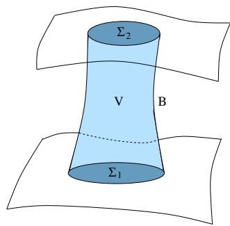
where B is the cylindrical timelike hypersurface.

We require that $J=0$ on B, which is the statement that no current flows in or out of the region. Then we have

$$Q_e({\Sigma }_1)-Q_e({\Sigma }_2)={\int }_{{\Sigma }_1}\star J-{\int }_{{\Sigma }_2}\star J={\int }_{\partial V}\star J={\int }_{V}d\star J=0$$

which tells us that the electric charge remains constant in time.

Maxwell Equations Using Connections

The form of the Maxwell equations given above makes no reference to a connection. It does, however, use the metric, buried in the definition of the Hodge ⋆.

There is an equivalent formulation of the Maxwell equation using the covariant derivative. This will also serve to highlight the relationship between the covariant and exterior derivatives. First note that, given a one-form $A\in {\Lambda }^1(M)$ , we can define the field strength as

$$F_{\mu \nu }={\nabla }_{\mu }{A}_{\nu }-{\nabla }_{\nu }{A}_{\mu }={\partial }_{\mu }{A}_{\nu }-{\partial }_{\nu }{A}_{\mu }$$

where the Christoffel symbols have cancelled out by virtue of the anti-symmetry. This is what allowed us to define the exterior derivative without the need for a connection.

Next, consider the current one-form J. We can recast the statement of current conservation as follows:

Claim

$$d\star J=0\iff {\nabla }_{\mu }{J}^{\mu }=0$$

Proof

We have

$${\nabla }_{\mu }{J}^{\mu }={\partial }_{\mu }{J}^{\mu }+{\Gamma }_{\mu \rho }^{\mu }{J}^{\rho }=\frac{1}{\sqrt{-g}}{\partial }_{\mu }\left(\sqrt{-g}{J}^{\mu }\right)$$

where, in the second equality, we have used our previous result (3.21): ${\Gamma }_{\mu \nu }^{\mu }={\partial }_{\nu }$ log $\sqrt{|g|}$ But this final form is proportional to $d\star J$ , with the Hodge dual defined in (3.5). □

As an aside, in Riemannian signature the formula

$${\nabla }_{\mu }{J}^{\mu }=\frac{1}{\sqrt{g}}{\partial }_{\mu }(\sqrt{g}{J}^{\mu })$$

provides a quick way of computing the divergence in different coordinate systems (if you don’t have the inside cover of Jackson to hand). For example, in spherical polar coordinates on ${\mathbf{R}}^3$ , we have $g=r^4{\sin }^2\theta$ . Plug this into the expression above to immediately find

$$\nabla \cdot \mathbf{J}=\frac{1}{r^2}{\partial }_r(r^2{J}^r)+\frac{1}{\sin \theta }{\partial }_{\theta }(\sin \theta J^{\theta })+{\partial }_{\varphi }{J}^{\varphi }$$

The Maxwell equation (3.22) can also be written in terms of the covariant derivative

Claim

$$d\star F=\star J\iff {\nabla }_{\mu }{F}^{\mu \nu }=J^{\nu }\text{\hspace{1em}(3.24)}$$

Proof

We have

$$\begin{array}{rl}& {\nabla }_{\mu }{F}^{\mu \nu }={\partial }_{\mu }{F}^{\mu \nu }+{\Gamma }_{\mu \rho }^{\mu }{F}^{\rho \nu }+{\Gamma }_{\mu \rho }^{\nu }{F}^{\mu \rho }\\ & =\frac{1}{\sqrt{-g}}{\partial }_{\mu }(\sqrt{-g}{F}^{\mu \nu })+{\Gamma }_{\mu \rho }^{\nu }{F}^{\mu \rho }=\frac{1}{\sqrt{-g}}{\partial }_{\mu }(\sqrt{-g}{F}^{\mu \nu })\end{array}$$

where, in the second equality, we’ve again used (3.21) and in the final equality we’ve used the fact that ${\Gamma }_{\mu \rho }^{\nu }$ is symmetric while $F^{\mu \rho }$ is anti-symmetric. To complete the proof, you need to chase down the definitions of the Hodge dual (3.5) and the exterior derivative (2.26). (If you’re struggling to match factors of $\sqrt{-g}$ , then remember that the volume form $v=\sqrt{-g}ϵ$ is a tensor, while the epsilon symbol ${ϵ}_{{\mu }_1\dots {\mu }_4}$ is a tensor density.) □

来源与版本

正文：英文 · OCR 机器稿 · 待校对

核对状态：OCR 机器稿 · 待校对

原书 PDF

来源版本：michaelmas-2019-source-20260923

来源 PDF SHA-256：3ba65dc61f22a69c7d5fdf3e8e1f641efbfa6cf49a44b3dcb0fd5367ba9fcf1c

OCR 来源 SHA-256：4489f366864dc6e3f68337328d72571d937e8794fa6c9c377869436e2ed366c5

OCR 产物 SHA-256：38b6b4b78f944efdd02f8c297351892b846c7d7c2418f01413932926005b0acb