2.4 Homeomorphisms and topological invariants

2.4.1 Homeomorphisms

As we mentioned at the beginning of this chapter, the main purpose of topology is to classify spaces. Suppose we have several figures and ask ourselves which are equal and which are different. Since we have not defined what is meant by equal or different, we may say ‘they are all different from each other’ or ‘they are all the same figures’. Some of the definitions of equivalence are too stringent and some are too loose to produce any sensible classification of the figures or spaces. For example, in elementary geometry, the equivalence of figures is given by congruence, which turns out to be too stringent for our purpose. In topology, we define two figures to be equivalent if it is possible to deform one figure into the other by continuous deformation. Namely we introduce the equivalence relation under which geometrical objects are classified according to whether it is possible to deform one object into the other by continuous deformation. To be more mathematical, we need to introduce the following notion of homeomorphism.

Definition 2.9

Let $X_1$ and $X_2$ be topological spaces. A map $f:X_1\to X_2$ is a homeomorphism if it is continuous and has an inverse $f^{-1}:X_2\to X_1$ which is also continuous. If there exists a homeomorphism between $X_1$ and $X_2$ , $X_1$ is said to be homeomorphic to $X_2$ and vice versa.

In other words, $X_1$ is homeomorphic to $X_2$ if there exist maps $f:X_1\to X_2$ and $g:X_2\to X_1$ such that $f\circ g={\mathrm{id}}_{X_2}$ , and $g\circ f={\mathrm{id}}_{X_1}$ . It is easy to show that a homeomorphism is an equivalence relation. Reflectivity follows from the choice $f={\mathrm{id}}_X$ , while symmetry follows since if $f:X_1\to X_2$ is a homeomorphism so is $f^{-1}:X_2\to X_1$ by definition. Transitivity follows since, if $f:X_1\to X_2$ and $g:X_2\to X_3$ are homeomorphisms so is $g\circ f:X_1\to X_3$ . Now we divide all topological spaces into equivalence classes according to whether it is possible to deform one space into the other by a homeomorphism. Intuitively speaking, we suppose the topological spaces are made out of ideal rubber which we can deform at our will. Two topological spaces are homeomorphic to each other if we can deform one into the other continuously, that is, without tearing them apart or pasting.

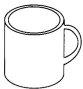
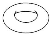
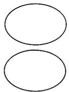
Figure 2.10 shows some examples of homeomorphisms. It seems impossible to deform the left figure in figure $2.10(b)$ into the right one by continuous deformation. However, this is an artefact of the embedding of these objects in ${\mathbb{R}}^3$ . In fact, they are continuously deformable in ${\mathbb{R}}^4$ , see problem 2.3. To distinguish one from the other, we have to embed them in $S^3$ , say, and compare the complements of these objects in $S^3$ . This approach is, however, out of the scope of the present book and we will content ourselves with homeomorphisms.

(a)

(b)

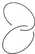
Figure 2.10. (a) A coffee cup is homeomorphic to a doughnut. (b) The linked rings are homeomorphic to the separated rings.

2.4.2 Topological invariants

Now our main question is: ‘How can we characterize the equivalence classes of homeomorphism?’ In fact, we do not know the complete answer to this question yet. Instead, we have a rather modest statement, that is, if two spaces have different ‘topological invariants’, they are not homeomorphic to each other. Here topological invariants are those quantities which are conserved under homeomorphisms. A topological invariant may be a number such as the number of connected components of the space, an algebraic structure such as a group or

a ring which is constructed out of the space, or something like connectedness, compactness or the Hausdorff property. (Although it seems to be intuitively clear that these are topological invariants, we have to prove that they indeed are. We omit the proofs. An interested reader may consult any text book on topology.) If we knew the complete set of topological invariants we could specify the equivalence class by giving these invariants. However, so far we know a partial set of topological invariants, which means that even if all the known topological invariants of two topological spaces coincide, they may not be homeomorphic to each other. Instead, what we can say at most is: if two topological spaces have different topological invariants they cannot be homeomorphic to each other.

Example 2.13

(a) A closed line $[-1,1]$ is not homeomorphic to an open line $(-1,1)$ , since $[-1,1]$ is compact while $(-1,1)$ is not.

(b) A circle $S^1$ is not homeomorphic to $\mathbb{R}$ , since $S^1$ is compact in ${\mathbb{R}}^2$ while $\mathbb{R}$ is not.
(c) A parabola $(y=x^2)$ is not homeomorphic to a hyperbola $(x^2-y^2=1)$ although they are both non-compact. A parabola is (arcwise) connected while a hyperbola is not.
(d) A circle $S^1$ is not homeomorphic to an interval $[-1,1]$ , although they are both compact and (arwise) connected. $[-1,1]$ is simply connected while $S^1$ is not. Alternatively $S^1-\{p\}$ , $p$ being any point in $S^1$ is connected while $[-1,1]-\{0\}$ is not, which is more evidence against their equivalence.
(e) Surprisingly, an interval without the endpoints is homeomorphic to a line $\mathbb{R}$ . To see this, let us take $X=(-\pi /2,\pi /2)$ and $Y=\mathbb{R}$ and let $f:X\to Y$ be $f(x)=\tan x$ . Since $\tan x$ is one to one on $X$ and has an inverse, ${\tan }^{-1}x$ , which is one to one on $\mathbb{R}$ , this is indeed a homeomorphism. Thus, boundedness is not a topological invariant.
(f) An open disc $D^2=\{(x,y)\in {\mathbb{R}}^2|x^2+y^2<1\}$ is homeomorphic to ${\mathbb{R}}^2$ . A homeomorphism $f:D^2\to {\mathbb{R}}^2$ may be

$$f(x,y)=\left(\frac{x}{\sqrt{1-x^2-y^2}},\frac{y}{\sqrt{1-x^2-y^2}}\right)\text{\hspace{1em}(2.28)}$$

while the inverse $f^{-1}:{\mathbb{R}}^2\to D^2$ is

$$f^{-1}(x,y)=\left(\frac{x}{\sqrt{1+x^2+y^2}},\frac{y}{\sqrt{1+x^2+y^2}}\right).\text{\hspace{1em}(2.29)}$$

The reader should verify that $f\circ f^{-1}={\mathrm{id}}_{{\mathbb{R}}^2}$ , and $f^{-1}\circ f={\mathrm{id}}_{D^2}$ . As we saw in example 2.5(e), a closed disc whose boundary $S^1$ corresponds to a point is homeomorphic to $S^2$ . If we take this point away, we have an open disc. The present analysis shows that this open disc is homeomorphic to ${\mathbb{R}}^2$ . By reversing the order of arguments, we find that if we add a point (infinity) to ${\mathbb{R}}^2$ , we obtain a compact space $S^2$ . This procedure is the one-point compactification $S^2={\mathbb{R}}^2\cup \{\infty \}$ introduced in the previous section. We similarly have $S^n={\mathbb{R}}^n\cup \{\infty \}$ .

(g) A circle $S^1=\{(x,y)\in {\mathbb{R}}^2|x^2+y^2=1\}$ is homeomorphic to a square $I^2=\{(x,y)\in {\mathbb{R}}^2|(|x|=1,|y|\le 1),(|x|\le 1,|y|=1)\}$ . A homeomorphism $f:I^2\to S^1$ may be given by

$$f(x,y)=\left(\frac{x}{r},\frac{y}{r}\right)r=\sqrt{x^2+y^2}.\text{\hspace{1em}(2.30)}$$

Since $r$ cannot vanish, (2.27) is invertible.

Exercise 2.18

Find a homeomorphism between a circle $S^1=\{(x,y)\in {\mathbb{R}}^2|x^2+y^2=1\}$ and an ellipse $E=\{(x,y)\in {\mathbb{R}}^2|(x/a{)}^2+(y/b{)}^2=1\}$ .

2.4.3 Homotopy type

An equivalence class which is somewhat coarser than homeomorphism but which is still quite useful is ‘of the same homotopy type’. We relax the conditions in definition 2.9 so that the continuous functions $f$ or $g$ need not have inverses. For example, take $X=(0,1)$ and $Y=\{0\}$ and let $f:X\to Y$ , $f(x)=0$ and $g:Y\to X$ , $g(0)=\frac{1}{2}$ . Then $f\circ g={\mathrm{id}}_Y$ , while $g\circ f\ne {\mathrm{id}}_X$ . This shows that an open interval $(0,1)$ is of the same homotopy type as a point $\{0\}$ , although it is not homeomorphic to $\{0\}$ . We have more on this topic in section 4.2.

Example 2.14

(a) $S^1$ is of the same homotopy type as a cylinder, since a cylinder is a direct product $S^1\times \mathbb{R}$ and we can shrink $\mathbb{R}$ to a point at each point of $S^1$ . By the same reason, the Möbius strip is of the same homotopy type as $S^1$ .

(b) A disc $D^2=\{(x,y)\in {\mathbb{R}}^2|x^2+y^2<1\}$ is of the same homotopy type as a point. $D^2-\{(0,0)\}$ is of the same homotopy type as $S^1$ . Similarly, ${\mathbb{R}}^2-\{0\}$ is of the same homotopy type as $S^1$ and ${\mathbb{R}}^3-\{0\}$ as $S^2$ .

2.4.4 Euler characteristic: an example

The Euler characteristic is one of the most useful topological invariants. Moreover, we find the prototype of the algebraic approach to topology in it. To avoid unnecessary complication, we restrict ourselves to points, lines and surfaces in ${\mathbb{R}}^3$ . A polyhedron is a geometrical object surrounded by faces. The boundary of two faces is an edge and two edges meet at a vertex. We extend the definition of a polyhedron a bit to include polygons and the boundaries of polygons, lines or points. We call the faces, edges and vertices of a polyhedron simplexes. Note that the boundary of two simplexes is either empty or another simplex. (For example, the boundary of two faces is an edge.) Formal definitions of a simplex and a polyhedron in a general number of dimensions will be given in chapter 3. We are now ready to define the Euler characteristic of a figure in ${\mathbb{R}}^3$ .

Definition 2.10

Let $X$ be a subset of ${\mathbb{R}}^3$ , which is homeomorphic to a polyhedron $K$ . Then the Euler characteristic $\chi (X)$ of $X$ is defined by

$$\begin{array}{rl}& \chi (X)=(\text{n u m b e r o f v e r t i c i e s i n}K)-(\text{n u m b e r o f e d g e s i n}K)\\ & +(\text{n u m b e r o f f a c e s i n}K).\end{array}\text{\hspace{1em}(2.31)}$$

The reader might wonder if $\chi (X)$ depends on the polyhedron $K$ or not. The following theorem due to Poincaré and Alexander guarantees that it is, in fact, independent of the polyhedron $K$ .

Theorem 2.4 · Poincaré-Alexander

The Euler characteristic $\chi (X)$ is independent of the polyhedron $K$ as long as $K$ is homeomorphic to $X$ .

Examples are in order. The Euler characteristic of a point is $\chi (\cdot )=1$ by definition. The Euler characteristic of a line is $\chi (⟶)=2-1=1$ , since a line has two vertices and an edge. For a triangular disc, we find $\chi (\text{triangle})=3-3+1=1$ . An example which is a bit non-trivial is the Euler characteristic of $S^1$ . The simplest polyhedron which is homeomorphic to $S^1$ is made of three edges of a triangle. Then $\chi (S^1)=3-3=0$ . Similarly, the sphere $S^2$ is homeomorphic to the surface of a tetrahedron, hence $\chi (S^2)=4-6+4=2$ . It is easily seen that $S^2$ is also homeomorphic to the surface of a cube. Using a cube to calculate the Euler characteristic of $S^2$ , we have $\chi (S^2)=8-12+6=2$ , in accord with theorem 2.4. Historically this is the conclusion of Euler’s theorem: if $K$ is any polyhedron homeomorphic to $S^2$ , with $v$ vertices, $e$ edges and $f$ two-dimensional faces, then $v-e+f=2$ .

Example 2.15

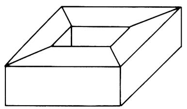
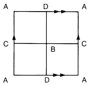
Let us calculate the Euler characteristic of the torus $T^2$ . Figure 2.11(a) is an example of a polyhedron which is homeomorphic to $T^2$ . From this polyhedron, we find $\chi (T^2)=16-32+16=0$ . As we saw in example 2.5(b), $T^2$ is equivalent to a rectangle whose edges are identified; see figure 2.4. Taking care of this identification, we find an example of a polyhedron made of rectangular faces as in figure 2.11(b), from which we also have $\chi (T^2)=0$ . This approach is quite useful when the figure cannot be realized (embedded) in ${\mathbb{R}}^3$ . For example, the Klein bottle (figure 2.5(a)) cannot be realized in ${\mathbb{R}}^3$ without intersecting itself. From the rectangle of figure 2.5(a), we find $\chi (\text{Klein bottle})=0$ . Similarly, we have $\chi (\text{projective plane})=1$ .

(a)

(b)

Figure 2.11. Example of a polyhedron which is homeomorphic to a torus.

Exercise 2.19

(a) Show that $\chi (\text{Mo¨bius strip})=0$ .

(b) Show that $\chi ({\Sigma }_2)=-2$ , where ${\Sigma }_2$ is the torus with two handles (see example 2.5). The reader may either construct a polyhedron homeomorphic to ${\Sigma }_2$ or make use of the octagon in figure 2.6(a). We show later that $\chi ({\Sigma }_g)=2-2g$ , where ${\Sigma }_g$ is the torus with $g$ handles.

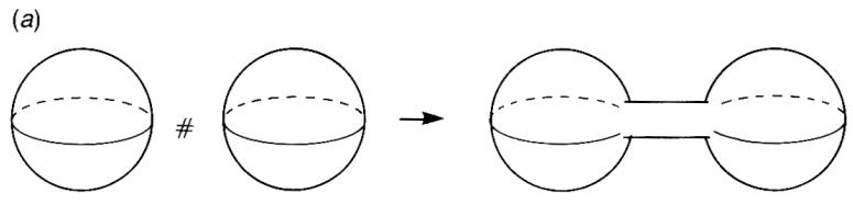
The connected sum $X♯Y$ of two surfaces $X$ and $Y$ is a surface obtained by removing a small disc from each of $X$ and $Y$ and connecting the resulting holes with a cylinder; see figure 2.12. Let $X$ be an arbitrary surface. Then it is easy to see that

Figure 2.12. The connected sum. (a) $S^2♯S^2=S2$ , (b) $T^2♯T^2={\Sigma }_2$ .

$$S^2♯X=X\text{\hspace{1em}(2.32)}$$

since $S^2$ and the cylinder may be deformed so that they fill in the hole on $X$ ; see figure 2.12(a). If we take a connected sum of two tori we get (figure 2.12(b))

$$T^2♯T^2={\Sigma }_2.\text{\hspace{1em}(2.33)}$$

Similarly, ${\Sigma }_g$ may be given by the connected sum of $g$ tori,

$$\underset{g\text{f a c t o r s}}{\underbrace{T^2♯T^2♯\cdots ♯T^2}}={\Sigma }_g.\text{\hspace{1em}(2.34)}$$

The connected sum may be used as a trick to calculate an Euler characteristic of a complicated surface from those of known surfaces. Let us prove the following theorem.

Theorem 2.5

Let $X$ and $Y$ be two surfaces. Then the Euler characteristic of the connected sum $X♯Y$ is given by

$$\chi (X♯Y)=\chi (X)+\chi (Y)-2.$$

Proof

Take polyhedra $K_X$ and $K_Y$ homeomorphic to $X$ and $Y$ , respectively. We assume, without loss of generality, that each of $K_Y$ and $K_Y$ has a triangle in it. Remove the triangles from them and connect the resulting holes with a trigonal cylinder. Then the number of vertices does not change while the number of edges increases by three. Since we have removed two faces and added three faces, the number of faces increases by $-2+3=1$ . Thus, the change of the Euler characteristic is $0-3+1=-2$ .

From the previous theorem and the equality $\chi (T^2)=0$ , we obtain $\chi ({\Sigma }_2)=0+0-2=-2$ and $\chi ({\Sigma }_g)=g\times 0-2(g-1)=2-2g$ , cf exercise 2.19(b).

The significance of the Euler characteristic is that it is a topological invariant, which is calculated relatively easily. We accept, without proof, the following theorem.

Theorem 2.6

Let $X$ and $Y$ be two figures in ${\mathbb{R}}^3$ . If $X$ is homeomorphic to $Y$ , then $\chi (X)=\chi (Y)$ . In other words, if $\chi (X)\ne \chi (Y)$ , $X$ cannot be homeomorphic to $Y$ .

Example 2.16

(a) $S^1$ is not homeomorphic to $S^2$ , since $\chi (S^1)=0$ while $\chi (S^2)=2$ .

(b) Two figures, which are not homeomorphic to each other, may have the same Euler characteristic. A point $(\cdot )$ is not homeomorphic to a line $(⟶)$ but $\chi (\cdot )=\chi (⟶)=1$ . This is a general consequence of the following fact: if a figure $X$ is of the same homotopy type as a figure $Y$ , then $\chi (X)=\chi (Y)$ .

The reader might have noticed that the Euler characteristic is different from other topological invariants such as compactness or connectedness in character. Compactness and connectedness are geometrical properties of a figure or a space while the Euler characteristic is an integer $\chi (X)\in \mathbb{Z}$ . Note that $\mathbb{Z}$ is an algebraic object rather than a geometrical one. Since the work of Euler, many mathematicians have worked out the relation between geometry and algebra and elaborated this idea, in the last century, to establish combinatorial topology and algebraic topology. We may compute the Euler characteristic of a smooth surface by the celebrated Gauss-Bonnet theorem, which relates the integral of the Gauss curvature of the surface with the Euler characteristic calculated from the corresponding polyhedron. We will give the generalized form of the Gauss-Bonnet theorem in chapter 12.

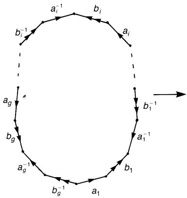
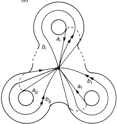
2.1 Show that the $4g$ -gon in figure 2.13(a), with the boundary identified, represents the torus with genus $g$ of figure 2.13(b). The reader may use equation (2.34).

(a)

Figure 2.13. The polygon $(a)$ whose edges are identified is the torus ${\Sigma }_g$ with genus $g$ .

(b)

2.2 Let $X=\{1,1/2,\dots ,1/n,\dots \}$ be a subset of $\mathbb{R}$ . Show that $X$ is not closed in $\mathbb{R}$ . Show that $Y=\{1,1/2,\dots ,1/n,\dots ,0\}$ is closed in $\mathbb{R}$ , hence compact.

2.3 Show that two figures in figure 2.109(b) are homeomorphic to each other. Find how to unlink the right figure in ${\mathbb{R}}^4$ . 2.4 Show that there are only five regular polyhedra: a tetrahedron, a hexahedron, an octahedron, a dodecahedron and an icosahedron. [Hint: Use Euler’s theorem.]

来源与版本

正文：英文 · OCR 机器稿 · 待校对

核对状态：OCR 机器稿 · 待校对

原书 PDF

来源版本：second-edition-local

来源 PDF SHA-256：fcd24c3371d092a8c699ccf5cf0765462924b6c48412804231076e8084b1940d

OCR 来源 SHA-256：0b6324f01172a3548cd34382e82fd8bfae574602b6b2cfaa357ba96bc2c35478

OCR 产物 SHA-256：a7e00021ffcc9683eabf608fae0184b3bd210e8d063798ebcadff51189fd7370