14.2 Quantum theory of bosonic strings

Now we are ready to introduce Polyakov’s formulation of bosonic strings, which is based on the path integral over geometries. Since the string action contains an enormous symmetry, we have to pay special attention to counting independent geometries once and only once. This is achieved by the Faddeev-Popov trick. Our argument will be restricted to the simplest case, namely closed orientable bosonic strings; the theory is defined on Riemann surfaces.

14.2.1 Vacuum amplitude of Polyakov strings

According to the general prescription of the path integral formalism, the partition function (vacuum-to-vacuum amplitude) of the string theory is given by

$$Z=\sum _{g=0}^{\infty }{Z}_g=\sum _{g=0}^{\infty }\int \mathcal{D}X\mathcal{D}\gamma {\mathrm{e}}^{-S[X,\gamma ]}\text{\hspace{1em}(14.30)}$$

see figure 14.1. To avoid confusion, we denote the genus by $g$ and the metric by $\gamma$ . The sum over genera amounts to the sum over the topologies. $Z_g$ is the $g$ -loop amplitude and is obtained by integrating over all metrics $\gamma$ and all embeddings $X$ . As we shall see later, the measure $\mathcal{D}X\mathcal{D}\gamma$ is not well defined and we need some modifications. The string action $S[X,\gamma ]$ is taken to be

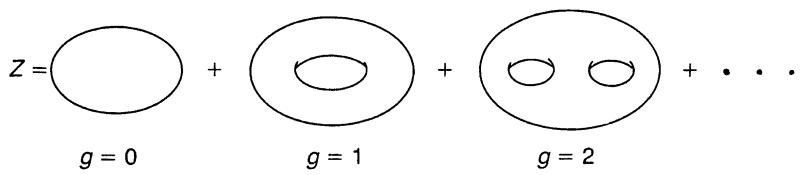
Figure 14.1. The total vacuum amplitude is given by summing over $g$ -loop amplitudes.

$$S[X,\gamma ]\equiv \frac{1}{2}\int {\mathrm{d}}^2\xi \sqrt{\gamma }{\gamma }^{\alpha \beta }{\partial }_{\alpha }{X}^{\mu }{\partial }_{\beta }{X}_{\mu }+\frac{\lambda }{4\pi }\int {\mathrm{d}}^2\xi \sqrt{\gamma }\mathcal{R}.\text{\hspace{1em}(14.31)}$$

The first term is the Polyakov action. The second term is proportional to the Euler characteristic

$$\chi =\frac{1}{4\pi }\int {\mathrm{d}}^2\xi \sqrt{\gamma }\mathcal{R}=2-2g$$

and serves as the string coupling constant; the amplitude of a loop with genus $g$ is suppressed by the factor ${\mathrm{e}}^{-2\lambda g}$ . Since this term is a topological invariant, it does not affect the dynamics of the string. We are interested in Riemann surfaces of a fixed genus $g$ and drop this term. The first term of the action has the following symmetries (section 7.11):

(A) $\mathrm{Diff}({\Sigma }_g)$ , the group of diffeomorphisms $f:{\Sigma }_g\to {\Sigma }_g$ . Let ${\xi }^{\alpha }\to {\xi }^{\prime \alpha }(\xi )$ be the coordinate expression for $f$ . The new metric is the pullback of the old one whose coordinate component expression is

$${\gamma }_{\alpha \beta }\to f^{\ast }{\gamma }_{\alpha \beta }=\frac{\partial {\xi }^{\gamma }}{\partial {\xi }^{\prime \alpha }}\frac{\partial {\xi }^{\delta }}{\partial {\xi }^{\prime \beta }}{\gamma }_{\gamma \delta }.\text{\hspace{1em}(14.32)}$$

The embedding also gets transformed as

$$X^{\mu }\to f^{\ast }{X}^{\mu }=X^{\mu }f.\text{\hspace{1em}(14.33)}$$

The invariance of the classical action takes the form

$$S[X,\gamma ]=S[f^{\ast }X,f^{\ast }\gamma ].\text{\hspace{1em}(14.34)}$$

(B) Weyl $({\Sigma }_g)$ , the group of two-dimensional Weyl rescalings

$${\gamma }_{\alpha \beta }\to {\hat{\gamma }}_{\alpha \beta }\equiv {\mathrm{e}}^{\varphi }{\gamma }_{\alpha \beta }\text{\hspace{1em}(14.35)}$$

where $\varphi \in \mathcal{F}({\Sigma }_g)$ . The conformal invariance of $S$ takes the form

$$S[X,\gamma ]=S[X,\hat{\gamma }].\text{\hspace{1em}(14.36)}$$

The symmetries (A) and (B) must be preserved under quantization, otherwise the theory has anomalies.

According to the standard Faddeev-Popov formalism, the degrees of freedom corresponding to these symmetries have to be omitted when we define $Z_g$ . For example, the string geometry specified by the pairs $(X_1,{\gamma }_1)$ and $(X_2,{\gamma }_2)$ should not be counted independently if they are related by an element of $\mathrm{Diff}({\Sigma }_g)$ . Similarly, $(X,\gamma )$ and $(X,{\mathrm{e}}^{\varphi }\gamma )$ should not be counted as independent configurations. Unless special attention is paid, we would count the same configurations infinitely many times, which leads to disastrous divergences. It turns out that the space of all the geometries $(X,\gamma )$ can be separated into equivalence classes (the gauge slice), any two points of which cannot be connected by these symmetries, see figure 14.2.

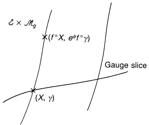
Figure 14.2. An element of $\mathcal{E}\times {\mathcal{M}}_g$ is obtained by the action of $\mathrm{Diff}({\Sigma }_g)\ast \mathrm{Weyl}({\Sigma }_g)$ on an element $(X,\gamma )$ in the gauge slice.

To be more mathematical, let $\mathcal{E}$ be the space of all the embeddings $X:{\Sigma }_g\to {\mathbb{R}}^D$ and let ${\mathcal{M}}_g$ be the space of all the metrics defined on ${\Sigma }_g$ . Naively, the path integral is defined over $\mathcal{E}\times {\mathcal{M}}_g$ . Because of the symmetries (A) and (B), however, the integral should be restricted to the quotient space $(\mathcal{E}\times {\mathcal{M}}_g)/G$ where $G=\mathrm{Diff}({\Sigma }_g)\ast \mathrm{Weyl}({\Sigma }_g)$ is the gauge group. The action of $(f,{\mathrm{e}}^{\varphi })$ on $(X,\gamma )\in \mathcal{E}\times {\mathcal{M}}_g$ is

$$(f,{\mathrm{e}}^{\varphi })(X,\gamma )=\left(f^{\ast }X,{\mathrm{e}}^{\varphi }{f}^{\ast }\gamma \right).\text{\hspace{1em}(14.37)}$$

The quotient ${\mathcal{M}}_g/G$ is called the moduli space of ${\Sigma }_g$ and is denoted by $\mathrm{Mod}({\Sigma }_g)$ . We are also interested in the subgroup ${\mathrm{Diff}}_0({\Sigma }_g)$ of $\mathrm{Diff}({\Sigma }_g)$ , which

is a connected component of the identity map. The quotient space $\mathrm{Teich}({\Sigma }_g)\equiv {\mathcal{M}}_g/{\mathrm{Diff}}_0({\Sigma }_g)\ast \mathrm{Weyl}({\Sigma }_g)$ is called the Teichmüller space of ${\Sigma }_g$ . The general theory of Riemann surfaces shows that $\mathrm{Teich}({\Sigma }_g)$ is a finite-dimensional universal covering space of $\mathrm{Mod}({\Sigma }_g)$ . Explicitly, we have

$${\dim }_{\mathbb{R}}\mathrm{Teich}\left({\Sigma }_{\mathrm{g}}\right)=\{\begin{array}{ll}0& g=0\\ 2& g=1\\ 6g-6& g\ge 2.\end{array}\text{\hspace{1em}(14.38)}$$

The group $\mathrm{Diff}({\Sigma }_g)/{\mathrm{Diff}}_0({\Sigma }_g)$ is known as the modular group (MG) or the mapping class group (MCG). The MCG is generated by the Dehn twists defined in example 8.2. For the torus with genus $g$ , the MCG is generated by $3g-1$ Dehn twists around $a_i,b_i$ and $c_i$ in figure 14.3. Unfortunately, these $3g-1$ Dehn twists are not the minimal set of the generators. The general form of MCG for $g\ge 2$ is not well understood.

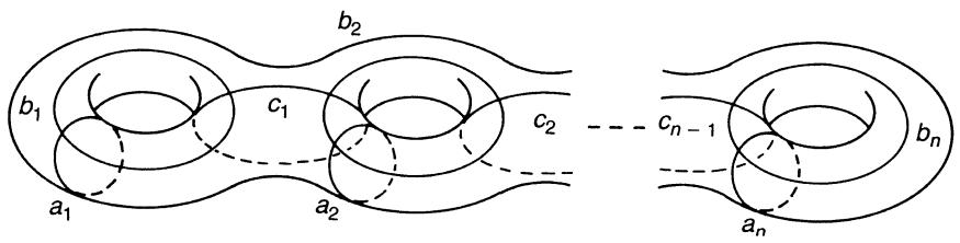
Figure 14.3. The mapping class group (MCG) is generated by Dehn twists around $a_i,b_i$ and $c_i$ ( $1\le i\le g$ ).

From these arguments, the meaningful partition function turns out to be

$$Z_{\mathrm{g}}\equiv {\int }_{\mathcal{E}\times {\mathcal{M}}_g}\frac{\mathcal{D}X\mathcal{D}\gamma }{V(\mathrm{Diff}\ast \mathrm{Weyl})}{\mathrm{e}}^{-S[X,\gamma ]}\text{\hspace{1em}(14.39)}$$

where $V(\mathrm{Diff}\ast \mathrm{Weyl})$ is the (infinite) volume of the space of $\mathrm{Diff}({\Sigma }_g)\ast \mathrm{Weyl}({\Sigma }_g)$ and takes care of the infinite overcounting of the same geometry. The order (the number of elements) of MCG is denoted by $|\mathrm{MCG}|$ . Clearly,

$$V(\text{D i f f}\ast \text{W e y l})=|\text{M C G}|V({\text{D i f f}}_0\ast \text{W e y l}).\text{\hspace{1em}(14.40)}$$

14.2.2 Measures of integration

We have to define a sensible measure to carry out the integration (14.39) so that the physical degrees of freedom and the gauge degrees of freedom are separated. This separation of degrees of freedom requires the Jacobian,

$$\mathcal{D}\gamma \mathcal{D}X\to J(\mathcal{D}\text{p h y s i c a l})(\mathcal{D}\text{g a u g e}).\text{\hspace{1em}(14.41)}$$

To find this Jacobian, we note that the Jacobian on a manifold $M$ agrees with that on $TM$ . To see this, let $x^{\mu }(y^{\mu })$ be a coordinate of a chart $U(V)$ of $M$ such that $U\cap V\ne \varnothing$ . The Jacobian of the coordinate change is $J=\det (\partial y^{\mu }/\partial x^{\nu })$ . Take $V\in T_{p}M$ . In components, we have $V=u^{\mu }\partial /\partial x^{\mu }=v^{\mu }\partial /\partial y^{\mu }$ , where

$$v^{\mu }=u^v\left(\partial y^{\mu }/\partial x^v\right).\text{\hspace{1em}(14.42)}$$

$\{u^{\mu }\}$ and $\{v^{\mu }\}$ are fibre coordinates of $T_{p}M$ . The Jacobian $\hat{J}$ associated with this coordinate change is

$$\hat{J}=\det \left(\partial v^{\mu }/\partial u^v\right)=\det \left(\partial y^{\mu }/\partial x^v\right)=J.\text{\hspace{1em}(14.43)}$$

This shows that the Jacobian at $p\in M$ is the same as that on $T_{p}M$ . The Jacobian $\hat{J}$ depends on $p$ but not on the vector itself, since $J$ depends only on $p$ .

Example 14.2

Let $(x,y)$ and $(r,\theta )$ be coordinates of ${\mathbb{R}}^2$ , where $x=r\cos \theta$ and $y=r\sin \theta$ . The Jacobian of the coordinate change is

$$J=\det \frac{\partial (x,y)}{\partial (r,\theta )}=r.$$

Let us take

$$V=v_x\partial /\partial x+v_y\partial /\partial y=v_r\partial /\partial r+v_{\theta }\partial /\partial \theta \in T_p{R}^2.$$

$(v_x,v_y)$ and $(v_r,v_{\theta })$ serve as fibre coordinates of $T_p{\mathbb{R}}^2$ . Since

$$v_x=v_r\partial x/\partial r+v_{\theta }\partial x/\partial \theta v_y=v_r\partial y/\partial r+v_{\theta }\partial y/\partial \theta$$

the associated Jacobian $\hat{J}$ is easily calculated to be

$$\hat{J}=\det [\partial (v_x,v_y)/\partial (v_r,v_{\theta })]=\left|\begin{array}{cc}\partial x/\partial r& \partial x/\partial \theta \\ \partial y/\partial r& \partial y/\partial \theta \end{array}\right|=J.$$

Let us derive this Jacobian in an indirect but suggestive way. We normalize the measure ${\mathrm{d}}^{2}v$ as

$$1=\int d^{2}v\exp \left(-\frac{1}{2}\Vert v{\Vert }^2\right)=\int d{v}_{x}d{v}_y\exp \left[-\frac{1}{2}\left(v_x^2+v_y^2\right)\right].$$

We also have $\Vert v^2{\Vert }^2=v_r^2+r^2{v}_{\theta }^2$ . Noting that the Jacobian is independent of $v_r$ and $v_{\theta }$ , we have

$$1=J\int \mathrm{d}{v}_r\mathrm{d}{v}_{\theta }\exp \left[-\frac{1}{2}\left(v_r^2+r^2{v}_{\theta }^2\right)\right]=J{r}^{-1}$$

4 This normalization of the measure differs by a constant factor from the conventional one.

from which we find $J=r$ . We use this procedure to find the functional measure of string theory.

This analysis enables us to write

$$\mathcal{D}\delta \gamma \mathcal{D}\delta X=J\mathcal{D}\delta (\text{p h y s i c a l})\mathcal{D}\delta (\text{g a u g e})\text{\hspace{1em}(14.44)}$$

where $\delta \gamma$ ( $\delta X$ ) is a small variation of the metric $\gamma$ (the embedding $X$ ) and is regarded as an element of $T_{\gamma }({\mathcal{M}}_g)$ ( $T_X\mathcal{E}$ ). The meaning of the RHS becomes clear in a moment.

Consider the diffeomorphism generated by an infinitesimal vector field $\delta v$ on ${\Sigma }_g$ . Since $\delta v$ is infinitesimal, it belongs to ${\mathrm{Diff}}_0({\Sigma }_g)$ rather than the full group $\mathrm{Diff}({\Sigma }_g)$ . The changes of the metric and the embedding under $\delta v$ are (see (7.120))

$${\delta }_{\mathrm{D}}{\gamma }_{\alpha \beta }={\left({\mathcal{L}}_{\delta v}\gamma \right)}_{\alpha \beta }={\nabla }_{\alpha }\delta v_{\beta }+{\nabla }_{\beta }\delta v_{\alpha }{\delta }_{\mathrm{D}}X=\delta v^{\alpha }{\partial }_{\alpha }X.\text{\hspace{1em}(14.45)}$$

The changes of $\gamma$ and $X$ under an infinitesimal Weyl rescaling ${\mathrm{e}}^{\delta \varphi }$ are

$${\delta }_{\mathrm{W}}{\gamma }_{\alpha \beta }=\delta \varphi {\gamma }_{\alpha \beta }{\delta }_{\mathrm{W}}X=0.\text{\hspace{1em}(14.46)}$$

These changes belong to unphysical (gauge) degrees of freedom. In general, a small change of metric is given by

$$\begin{array}{rl}\delta {\gamma }_{\alpha \beta }& ={\delta }_{\mathrm{W}}{\gamma }_{\alpha \beta }+{\delta }_{\mathrm{D}}{\gamma }_{\alpha \beta }+(\text{p h y s i c a l c h a n g e})\\ & =\delta \varphi {\gamma }_{\alpha \beta }+{\nabla }_{\alpha }\delta v_{\beta }+{\nabla }_{\beta }\delta v_{\alpha }+\delta t^i\frac{\partial }{\partial t^i}{\gamma }_{\alpha \beta }(t)\end{array}\text{\hspace{1em}(14.47)}$$

where the last term is called the Teichmüller deformation of the metric, which can neither be described by a diffeomorphism nor by a Weyl rescaling. As mentioned before, $\{i\}$ is a finite set, $1\le i\le n={\dim }_{\mathbb{R}}\mathrm{Teich}({\Sigma }_g)$ . It is convenient for later purposes to separate $\delta \gamma$ into a traceless part and a part with a non-zero trace. We write

$$\delta {\gamma }_{\alpha \beta }=\delta \bar{\varphi }{\gamma }_{\alpha \beta }+(P_1\delta v{)}_{\alpha \beta }+\delta t^i{T}_{i\alpha \beta }(t)\text{\hspace{1em}(14.48)}$$

where $T_{i\alpha \beta }$ is the traceless part of the Teichmüller deformation,

$$T_{i\alpha \beta }\equiv \frac{\partial {\gamma }_{\alpha \beta }}{\partial t^i}-\frac{1}{2}{\gamma }_{\alpha \beta }{\gamma }^{\gamma \delta }\frac{\partial {\gamma }_{\gamma \delta }}{\partial t^i}.\text{\hspace{1em}(14.49)}$$

The operator $P_1$ is defined by

$${\left(P_1\delta v\right)}_{\alpha \beta }\equiv {\nabla }_{\alpha }\delta v_{\beta }+{\nabla }_{\beta }\delta v_{\alpha }-{\gamma }_{\alpha \beta }\left({\nabla }_{\gamma }\delta v_{\gamma }\right)\text{\hspace{1em}(14.50)}$$

and picks up the traceless part of ${\delta }_{\mathrm{D}}{\gamma }_{\alpha \beta }$ while $\delta \bar{\varphi }$ is defined by

$$\delta \bar{\varphi }=\delta \varphi +\left({\nabla }_{\gamma }\delta v^{\gamma }+\mathrm{trace}\mathrm{part}\delta t\frac{\partial \gamma }{\partial t}\right)\text{\hspace{1em}(14.51)}$$

where we do not need the explicit form in the parentheses.

As for the embeddings, we consider the quotient $\mathcal{E}/\mathrm{Diff}({\Sigma }_g)$ . An arbitrary embedding $X$ is obtained by the action of $\mathrm{Diff}({\Sigma }_g)$ on some $\tilde{X}\in \mathcal{E}/\mathrm{Diff}({\Sigma }_g)$ . Then a small change of the embedding is expressed as

$$\delta X=\delta v^{\alpha }{\partial }_{\alpha }\tilde{X}+\delta \tilde{X}\text{\hspace{1em}(14.52)}$$

where the first term represents the change of $X$ generated by $\delta v$ while the second is not associated with diffeomorphisms. Now the measure should look like

$$\mathcal{D}\delta \gamma \mathcal{D}\delta X=J{\mathrm{d}}^{n}t\mathcal{D}\delta v\mathcal{D}\delta \varphi \mathcal{D}\delta \tilde{X}.\text{\hspace{1em}(14.53)}$$

To define the measure, we need to specify a metric on the tangent space, see example 14.2. We restrict ourselves to the so called ultralocal metric which is quadratic and depends on ${\gamma }_{\alpha \beta }$ but not on $\partial {\gamma }_{\alpha \beta }$ . Define a metric for symmetric second-rank tensors by

$$\Vert \delta h{\Vert }_{\gamma }^2=\int {\mathrm{d}}^2\xi \sqrt{\gamma }\left(G^{\alpha \beta \gamma \delta }+u{\gamma }^{\alpha \beta }{\gamma }^{\gamma \delta }\right)\delta h_{\alpha \beta }\delta h_{\gamma \delta }\text{\hspace{1em}(14.54a)}$$

where $u>0$ is an arbitrary constant and

$$G^{\alpha \beta \gamma \delta }\equiv {\gamma }^{\alpha \gamma }{\gamma }^{\beta \delta }+{\gamma }^{\alpha \delta }{\gamma }^{\beta \gamma }-{\gamma }^{\alpha \beta }{\gamma }^{\gamma \delta }.\text{\hspace{1em}(14.55)}$$

It is readily verified that $G$ is the projection operator to the traceless part (tr $G^{\alpha \beta \gamma \delta }\delta h_{\gamma \delta }={\gamma }_{\alpha \beta }{G}^{\alpha \beta \gamma \delta }\delta h_{\gamma \delta }=0$ ) while $u{\gamma }^{\alpha \beta }{\gamma }^{\gamma \delta }$ is that to the trace part. In a finite-dimensional manifold, a metric defines a natural volume element. In the present case, however, the measure cannot be defined explicitly and we have to define it implicitly in terms of the Gaussian integral (see example 14.2),

$$\int \mathcal{D}\delta h\exp \left(-\frac{1}{2}||\delta h|{|}_{\gamma }^2\right)=1.\text{\hspace{1em}(14.56a)}$$

Similarly, the metrics for a scalar $\delta \varphi$ , a vector $\delta v$ and a map $\delta X^{\mu }$ are defined by

$${\Vert \delta \varphi \Vert }_{\gamma }^2=\int d^2\xi \sqrt{\gamma }\delta {\varphi }^2\text{\hspace{1em}(14.54b)}$$

$${\Vert \delta v\Vert }_{\gamma }^2=\int d^2\xi \sqrt{\gamma }{\gamma }_{\alpha \beta }\delta v^{\alpha }\delta v^{\beta }\text{\hspace{1em}(14.54c)}$$

$$\Vert \delta X{\Vert }_{\gamma }^2=\int {\mathrm{d}}^2\xi \sqrt{\gamma }\delta X^{\mu }\delta X_{\mu }.\text{\hspace{1em}(14.54d)}$$

With these metrics, the measures are defined by

$$\int \mathcal{D}\delta \varphi \exp \left(-\frac{1}{2}||\delta \varphi |{|}_{\gamma }^2\right)=1\text{\hspace{1em}(14.56b)}$$

$$\int \mathcal{D}\delta v\exp \left(-\frac{1}{2}||\delta v|{|}_{\gamma }^2\right)=1\text{\hspace{1em}(14.56c)}$$

$$\int \mathcal{D}\delta X\exp \left(-\frac{1}{2}||\delta X|{|}_{\gamma }^2\right)=1.\text{\hspace{1em}(14.56d)}$$

Exercise 14.3

Show that $\Vert \delta \gamma {\Vert }_{\gamma }^2$ and $\Vert \delta X{\Vert }_{\gamma }^2$ are invariant under $\mathrm{Diff}({\Sigma }_g)$ but not under Weyl $({\Sigma }_g)$ . This is the possible origin of conformal anomalies, see (14.84).

Before we proceed further, we need to clarify the overlap between ${\mathrm{Diff}}_0({\Sigma }_g)$ and $\mathrm{Weyl}({\Sigma }_g)$ . Suppose $\delta v\in \ker P_1$ , that is,

$$P_1\delta v={\nabla }_{\alpha }\delta v_{\beta }+{\nabla }_{\beta }\delta v_{\alpha }-{\gamma }_{\alpha \beta }({\nabla }_{\gamma }\delta v^{\gamma })=0.\text{\hspace{1em}(14.57)}$$

We find, for such $\delta v$ , that ${\delta }_{\mathrm{D}}{\gamma }_{\alpha \beta }=({\nabla }_{\gamma }\delta v^{\gamma }){\gamma }_{\alpha \beta }$ . A vector $\delta v\in \ker P_1$ is identified with the conformal Killing vector (CKV), see section 7.7. It is important to note that ${\delta }_{\mathrm{D}}$ and ${\delta }_{\mathrm{W}}$ yield the same metric deformations if $\delta \varphi$ is taken to be ${\nabla }_{\gamma }\delta v^{\gamma }$ . Thus, the set of the CKVs is identified with the overlap between ${\mathrm{Diff}}_0({\Sigma }_g)$ and Weyl( ${\Sigma }_g$ ). Let there be $k$ independent CKVs on ${\Sigma }_g$ and denote these by ${\Phi }_s^{\alpha }(1\le s\le k)$ . It is known from the theory of Riemann surfaces that

$$k=\{\begin{array}{ll}6& g=0\\ 2& g=1\\ 0& g\ge 2.\end{array}\text{\hspace{1em}(14.58)}$$

We separate $\delta v$ into a part generated by the CKV, and its orthogonal complement, which we write as

$$\delta v^{\alpha }=\delta {\tilde{v}}^{\alpha }+\delta a^s{\Phi }_s^{\alpha }.\text{\hspace{1em}(14.59)}$$

The tangent vector $\delta X$ is also decomposed as

$$\delta X=\delta \tilde{X}+\delta {\tilde{v}}^{\alpha }{\partial }_{\alpha }{\tilde{X}}^{\mu }+\delta a^s{\Phi }_s^{\alpha }{\partial }_{\alpha }{\tilde{X}}^{\mu }.\text{\hspace{1em}(14.60)}$$

The functional measures now become

$$\mathcal{D}\delta \gamma \mathcal{D}\delta X\to J{\mathrm{d}}^n\delta t\mathcal{D}\delta \varphi \mathcal{D}\delta \tilde{v}{\mathrm{d}}^k\delta a\mathcal{D}\delta \tilde{X}\text{\hspace{1em}(14.61)}$$

where we noted that the $t$ - and $a$ -parameters are finite dimensional.

Let ${\mathrm{Diff}}_0^{\perp }({\Sigma }_g)$ be the subspace of ${\mathrm{Diff}}_0({\Sigma }_g)$ , which is orthogonal to the CKV. We have

$$V\left({\mathrm{Diff}}_0\right)=V\left({\mathrm{Diff}}_0^{\perp }\right)\cdot V(\mathrm{CKV})\text{\hspace{1em}(14.62)}$$

$$\begin{array}{rl}V\left({\mathrm{Diff}}_0\ast \mathrm{Weyl}\right)& =V\left({\mathrm{Diff}}_0^{\perp }\right)V(\mathrm{Weyl})\\ & =V\left({\text{D i f f}}_0\right)V\left(\text{W e y l}\right)/V(\text{C K V}).\end{array}\text{\hspace{1em}(14.63)}$$

Take a slice $\hat{\gamma }(t)$ of ${\mathcal{M}}_g$ . The slice is parametrized by $n$ Teichmüller parameters. Any metric $\tilde{\gamma }$ related to $\hat{\gamma }$ by $G=\mathrm{Diff}({\Sigma }_g)\ast \mathrm{Weyl}({\Sigma }_g)$ is written as

$$\tilde{\gamma }=f^{\ast }\left({\mathrm{e}}^{\varphi }\hat{\gamma }\right)f\in \mathrm{Diff}\left({\Sigma }_g\right),{\mathrm{e}}^{\varphi }\in \mathrm{Weyl}\left({\Sigma }_g\right).\text{\hspace{1em}(14.64)}$$

We express a small deformation $\delta \tilde{\gamma }$ at $\tilde{\gamma }$ as a pullback of a deformation $\delta \gamma$ at $\gamma \equiv {\mathrm{e}}^{\delta \varphi }\hat{\gamma }$ : $\delta \tilde{\gamma }=f^{\ast }(\delta \gamma )$ . Note that $\delta \gamma$ is a small diffeomorphism at the origin

of ${\mathrm{Diff}}_0({\Sigma }_g)$ and, hence, can be described by a vector field $\delta v$ . As was shown in exercise 14.3, $\mathrm{Diff}({\Sigma }_g)$ is the isometry of the relevant vector spaces. It then follows that

$${\Vert \delta \tilde{\gamma }\Vert }_{\tilde{\gamma }}^2={\Vert f^{\ast }(\delta \gamma )\Vert }_{f^{\ast }\gamma }^2={\Vert \delta \gamma \Vert }_{\gamma }^2\gamma =e^{\varphi }\hat{\gamma }.\text{\hspace{1em}(14.65)}$$

At the point $\gamma$ , we decompose $\delta \gamma$ as

$$\delta {\gamma }_{\alpha \beta }=\delta \varphi {\gamma }_{\alpha \beta }+{\left(P_1\delta \tilde{v}\right)}_{\alpha \beta }+\delta t^i{T}_{i\alpha \beta }\text{\hspace{1em}(14.66)}$$

where $\delta \varphi$ has been redefined so that it includes the trace parts of the Teichmüller deformation and ${\nabla }_{\alpha }\delta v_{\beta }+{\nabla }_{\beta }\delta v_{\alpha }$ , see (14.51).

Exercise 14.4

Show that $T_{i\alpha \beta }$ at $\gamma$ is related to ${\hat{T}}_{i\alpha \beta }$ at $\hat{\gamma }$ as

$$T_{i\alpha \beta }={\mathrm{e}}^{\varphi }{\hat{T}}_{i\alpha \beta }.\text{\hspace{1em}(14.67)}$$

Now we are ready to give the explicit form of the measure. We first find the Jacobian associated with the change $\mathcal{D}\delta v\to \mathcal{D}\delta \tilde{v}{\mathrm{d}}^k\delta a$ . We have

$$\begin{array}{rl}1& =\int \mathcal{D}\delta v\exp \left(-\frac{1}{2}\Vert \delta v{\Vert }_{\gamma }^2\right)\\ & =J\int \mathcal{D}\delta \tilde{v}{d}^k\delta a\exp \left(-\frac{1}{2}\Vert \delta \tilde{v}{\Vert }_{\gamma }^2-\frac{1}{2}\Vert \delta a^s{\Phi }_s{\Vert }_{\gamma }^2\right)\\ & =J{\left[\det \left({\Phi }_s,{\Phi }_r\right)\right]}^{-1/2}\end{array}\text{\hspace{1em}(14.68a)}$$

where

$$\left({\Phi }_s,{\Phi }_r\right)=\int {\mathrm{d}}^2\xi \sqrt{\gamma }{\gamma }_{\alpha \beta }{\Phi }_s^{\alpha }{\Phi }_r^{\beta }.\text{\hspace{1em}(14.68b)}$$

[Remark: Although the matrix element (14.68b) is defined for $\gamma ={\mathrm{e}}^{\varphi }\hat{\gamma }$ , we can show that it is independent of ${\mathrm{e}}^{\varphi }$ . To see this, let us take a CKV ${\hat{\Phi }}_s^{\alpha }$ of the metric $\hat{\gamma }$ ; ${\hat{\nabla }}_{\alpha }{\hat{\Phi }}_{s\beta }+{\hat{\nabla }}_{\beta }{\hat{\Phi }}_{s\alpha }={\hat{\gamma }}_{\alpha \beta }\hat{\nabla }{\hat{\Phi }}_s^{\gamma }$ , where $\hat{\nabla }$ is the covariant derivative with respect to $\hat{\gamma }$ and ${\hat{\Phi }}_{s\alpha }\equiv {\hat{\gamma }}_{\alpha \beta }{\hat{\Phi }}_s^{\beta }$ . A simple calculation shows that ${\Phi }_{s\alpha }={\gamma }_{\alpha \beta }{\hat{\Phi }}_s^{\beta }={\mathrm{e}}^{\varphi }{\hat{\Phi }}_{s\alpha }$ satisfies

$$\begin{array}{rl}{\nabla }_{\alpha }{\Phi }_{s\beta }+{\nabla }_{\beta }{\Phi }_{s\alpha }& =e^{\varphi }({\hat{\nabla }}_{\alpha }{\hat{\Phi }}_{s\beta }+{\hat{\nabla }}_{\beta }{\hat{\Phi }}_{s\alpha }+{\hat{\gamma }}_{\alpha \beta }{\Phi }_s^{\gamma }{\partial }_{\gamma }\varphi )\\ & ={\mathrm{e}}^{\varphi }{\hat{\gamma }}_{\alpha \beta }\left({\hat{\nabla }}_{\gamma }{\Phi }_s^{\gamma }+{\Phi }_s^{\gamma }{\partial }_{\gamma }\varphi \right)={\gamma }_{\alpha \beta }{\nabla }_{\gamma }{\Phi }_s^{\gamma }\end{array}$$

$\nabla$ being the covariant derivative with respect to $\gamma$ . Thus, ${\Phi }_s^{\alpha }={\hat{\Phi }}_s^{\alpha }$ is a CKV of the metric $\gamma ={\mathrm{e}}^{\varphi }\hat{\gamma }$ and the CKV are taken to be $\varphi$ independent.] Equation (14.68a) shows that

$$\mathcal{D}\delta v={\left[\det \left({\Phi }_r,{\Phi }_s\right)\right]}^{1/2}\mathcal{D}\delta \tilde{v}{d}^k\delta a.\text{\hspace{1em}(14.69)}$$

Now the total measure is written as

$$J{\left[\det \left({\Phi }_r,{\Phi }_s\right)\right]}^{1/2}{\mathrm{d}}^{n}t\mathcal{D}\delta \varphi \mathcal{D}\delta \tilde{v}{\mathrm{d}}^k\delta a\mathcal{D}\delta \tilde{X}\text{\hspace{1em}(14.70)}$$

where $J$ takes care of the rest of the variable changes.

The Jacobian $J$ is now obtained from (14.60), (14.66), (14.70) and the definition of the measures (14.56). We have

$$\begin{array}{rl}& 1=\int \mathcal{D}\delta \gamma \mathcal{D}\delta X\exp (-\frac{1}{2}||\delta \gamma |{|}_{\gamma }^2-\frac{1}{2}||\delta X|{|}_{\gamma }^2)\\ & =J\stackrel{1/2}{\det }(\Phi ,\Phi )\int {\mathrm{d}}^n\delta t\mathcal{D}\delta \tilde{v}\mathcal{D}\delta \varphi {\mathrm{d}}^k\delta a\mathcal{D}\delta \tilde{X}\\ & \times \exp [-\frac{1}{2}{\Vert \delta \varphi {\gamma }_{\alpha \beta }+(P_1\delta \tilde{v}{)}_{\alpha \beta }+\delta t^i\frac{\partial {\gamma }_{\alpha \beta }}{\partial t^i}\Vert }^2\\ & -\frac{1}{2}\Vert \delta \tilde{X}+\delta {\tilde{v}}^{\alpha }{\partial }_{\alpha }\tilde{X}+\delta a^s{\Phi }_s^{\alpha }{\partial }_{\alpha }\tilde{X}{\Vert }^2]\\ & =J\stackrel{1/2}{\det }(\Phi ,\Phi )\int {\mathrm{d}}^n\delta t\mathcal{D}\delta \tilde{v}\dots \exp \left(-\frac{1}{2}\Vert MV{\Vert }^2\right)\end{array}\text{\hspace{1em}(14.71)}$$

where

$$V=\left(\begin{array}{l}\delta t\\ \delta \varphi \\ \delta \tilde{v}\\ \delta a\\ \delta \tilde{X}\end{array}\right)M=\left(\begin{array}{ccccc}\partial \gamma /\partial t& \gamma & P_1& 0& 0\\ 0& 0& \partial \tilde{X}& \Phi \cdot \partial \tilde{X}& 1\end{array}\right)\equiv \left(\begin{array}{cc}A& 0\\ C& B\end{array}\right).\text{\hspace{1em}(14.72)}$$

The matrix in the exponent of (14.71) is

$$\begin{array}{rl}{M}^{†}M& =\left(\begin{array}{cc}{A}^{†}& C^{†}\\ 0& B^{†}\end{array}\right)\left(\begin{array}{cc}A& 0\\ C& B\end{array}\right)=\left(\begin{array}{cc}{A}^{†}A+C^{†}C& C^{†}B\\ B^{†}C& B^{†}B\end{array}\right)\\ & =\left(\begin{array}{cc}I& \ast \\ 0& B^{†}B\end{array}\right)\left(\begin{array}{cc}{A}^{†}A& 0\\ \ast \ast & I\end{array}\right)\end{array}\text{\hspace{1em}(14.73)}$$

where $\ast$ and $\ast \ast$ are irrelevant. The last expression has been obtained from the identity,

$$\left(\begin{array}{cc}A& B\\ C& D\end{array}\right)=\left(\begin{array}{cc}I& B\\ 0& D\end{array}\right)\left(\begin{array}{cc}A-B{D}^{-1}C& 0\\ D^{-1}C& I\end{array}\right).$$

The Gaussian integrals in (14.71) are readily evaluated to yield

$$\begin{array}{rl}1& =J\stackrel{1/2}{\det }(\Phi ,\Phi )\stackrel{-1/2}{\det }(M^{†}M)\\ & =J\stackrel{1/2}{\det }(\Phi ,\Phi )[\det (A^{†}A)\det (B^{†}B){]}^{-1/2}.\end{array}\text{\hspace{1em}(14.74)}$$

To compute ${\det }^{1/2}(A^{†}A)$ , we need to evaluate $\Vert \delta \gamma {\Vert }_{\gamma }^2$ . We have

$$\begin{array}{rl}& ||\delta \gamma |{|}_{\gamma }^2=\int {\mathrm{d}}^2\xi \sqrt{\gamma }(G^{\alpha \beta \gamma \delta }+u{\gamma }^{\alpha \beta }{\gamma }^{\gamma \delta })\\ & \times [\delta \varphi {\gamma }_{\alpha \beta }+(P_1\delta \tilde{v}{)}_{\alpha \beta }+\delta t^i{T}_{i\alpha \beta }][\delta \varphi {\gamma }_{\gamma \delta }+(P_1\delta \tilde{v}{)}_{\gamma \delta }+\delta t^j{T}_{j\gamma \delta }]\\ & =4u\Vert \delta \varphi {\Vert }_{\gamma }^2+\Vert P_1\delta \tilde{v}{\Vert }^2+\delta t^i\delta t^j\left(T_i,T_j\right)+2\delta t^i\left(P_1\delta \tilde{v},T_i\right).\end{array}\text{\hspace{1em}(14.75)}$$

In general, $T_i$ is not orthogonal to $P_1\delta v$ . To separate $T_i$ into parts orthogonal to $P_1\delta v$ and parallel to $P_1\delta v$ , we need to define the adjoint $P_1^{†}$ of $P_1$ . $P_1$ is an elliptic operator which takes a vector field into a traceless symmetric tensor field. Thus, $P_1^{†}$ maps symmetric traceless tensors to vectors. For a symmetric traceless tensor $\delta h$ , we have

$$\begin{array}{rl}(P_1\delta v,\delta h)& =\int {\mathrm{d}}^2\xi \sqrt{\gamma }{G}^{\alpha \beta \gamma \delta }(P_1\delta v{)}_{\alpha \beta }\delta h_{\gamma \delta }\\ & =\int {\mathrm{d}}^2\xi \sqrt{\gamma }({\nabla }^{\alpha }\delta v^{\beta }+{\nabla }^{\beta }\delta v^{\alpha })\delta h_{\alpha \beta }\\ & =\int {\mathrm{d}}^2\xi \sqrt{\gamma }\delta v^{\alpha }(-2{\nabla }^{\beta })\delta h_{\alpha \beta }\equiv (\delta v,P_1^{†}\delta h)\end{array}$$

where the inner product in the last expression is defined by (14.54c). Thus, it follows that

$${\left(P_1^{†}\delta h\right)}_{\alpha }=-2{\nabla }^{\beta }\delta h_{\alpha \beta }.\text{\hspace{1em}(14.76)}$$

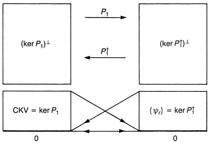
Suppose $\delta h$ is orthogonal to $P_1\delta v$ . From the previous discussion, we have $(P_1\delta v,\delta h)=(\delta v,P_1^{†}\delta h)=0$ . Since $\delta v$ is arbitrary, $\delta h$ must be an element of $\ker P_1^{†}$ , see figure 14.4. Now $T_i$ may be separated as

Figure 14.4. The map $P_1$ and its adjoint $P_1^{†}$ .

$$T_i={\mathcal{P}}_0{T}_i+{\mathcal{P}}_{\perp }{T}_i\text{\hspace{1em}(14.77a)}$$

where the projection operators ${\mathcal{P}}_0$ and ${\mathcal{P}}_{\perp }$ are defined by

$${\mathcal{P}}_0\equiv 1-P_1\frac{1}{P_1^{†}{P}_1}{P}_1^{†}{\mathcal{P}}_{\perp }\equiv P_1\frac{1}{P_1^{†}{P}_1}{P}_1^{†}.\text{\hspace{1em}(14.77b)}$$

It is easy to verify that ${\mathcal{P}}_0+{\mathcal{P}}_1=1$ , ${\mathcal{P}}_0{\mathcal{P}}_{\perp }=0$ , $P_1^{†}{\mathcal{P}}_0=0$ , $P_1^{†}{\mathcal{P}}_{\perp }=P_1^{†}$ , ${\mathcal{P}}_0{T}_i=T_i$ and ${\mathcal{P}}_{\perp }{T}_i=0$ for $T_i\in \ker P_1^{†}$ etc. Thus (14.77a) is an orthogonal decomposition of $T_i$ . We write ${\mathcal{P}}_{\perp }{T}_i=P_1{u}_i$ , where

$$u_i=\frac{1}{P_1^{†}{P}_1}{P}_1^{†}{T}_i.$$

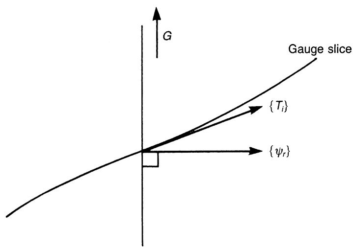
Let $\{{\psi }_r\}(1\le r\le n)$ be a real basis of $\ker P_1^{†}$ , which is not necessarily orthonormal. Then $T_i$ can be expanded as (figure 14.5)

Figure 14.5. $\{T_i\}$ spans the deformation tangent to the gauge slice while $\{{\psi }_r\}$ spans $\ker P_1^{†}$ .

$$T_i=\sum _r{\psi }_r{Q}_{ri}+P_1{u}_i.\text{\hspace{1em}(14.78)}$$

Taking an inner product between $T_i$ and ${\psi }_r$ , we find that

$$Q_{ri}=\sum _s[(\psi ,\psi {)}^{-1}{]}_{rs}\left({\psi }_s,T_i\right).\text{\hspace{1em}(14.79)}$$

Finally, $\delta \gamma$ is decomposed into mutually orthogonal pieces as

$$\delta \gamma =\delta \varphi \gamma +P_1\left(\delta \tilde{v}+\delta t^i{u}_i\right)+\delta t^i{\psi }_r{Q}_{ri}.\text{\hspace{1em}(14.80a)}$$

Correspondingly, the space of the metric deformation $\{\delta \gamma \}$ separates into the direct sum

$$\{\delta \gamma \}=\left\{\mathrm{conf}\right\}\oplus \left\{\mathrm{im}{P}_1\right\}\oplus \left\{\ker P_1^{†}\right\}.\text{\hspace{1em}(14.80b)}$$

Substituting (14.80a) into (14.75), we obtain

$$\begin{array}{rl}& {\left|\left|\delta \gamma \right|\right|}^2=4u{\left|\left|\delta \varphi \right|\right|}^2+{\left|\left|P_1\delta \bar{v}\right|\right|}^2\\ & +\delta t^i\delta t^j{\left(T_i,{\psi }_r\right)}_{\gamma }{\left[(\psi ,\psi {)}_{\gamma }^{-1}\right]}_{rs}{\left({\psi }_s,T_j\right)}_{\gamma }\end{array}\text{\hspace{1em}(14.81)}$$

where $\delta \bar{v}\equiv \delta \tilde{v}+\delta t^i{u}_i$ and the inverse in the last term refers to the inverse of the matrix $(a_{rs})=(({\psi }_r,{\psi }_s))$ . If we put ${\mathcal{V}}_1^t=(\delta t,\delta \varphi ,\delta \bar{v})$ , we find that

$$\begin{array}{rl}& \stackrel{-1/2}{\det }\left(A^{†}A\right)=\int {\mathrm{d}}^n\delta t\mathcal{D}\delta \varphi \mathcal{D}\delta \bar{v}\exp \left(-\frac{1}{2}{\mathcal{V}}_1^t{A}^{†}A{\mathcal{V}}_1\right)\\ & =\int \mathcal{D}\delta \varphi \exp (-2u||\delta \varphi |{|}^2)\int \mathcal{D}\delta \bar{v}\exp (-\frac{1}{2}||P_1\bar{v}|{|}^2)\\ & \times \int {\mathrm{d}}^n\delta t\exp \left\{-\frac{1}{2}\delta t^i\left(T_i,{\psi }_r\right){\left[(\psi ,\psi {)}^{-1}\right]}_{rs}\left({\psi }_s,T_j\right)\delta t^j\right\}\\ & \propto {\left(\det P_1^{†}{P}_1\right)}^{-1/2}{\left(\frac{\det (T,\psi {)}^2}{\det (\psi ,\psi )}\right)}^{-1/2}.\end{array}\text{\hspace{1em}(14.82)}$$

Collecting the results (14.71) and (14.82), we have

$$1=J\stackrel{1/2}{\det }(\Phi ,\Phi )\stackrel{-1/2}{\det }{B}^{†}B\stackrel{-1/2}{\det }{P}_1^{†}{P}_1{\left(\frac{\det (T,\psi {)}^2}{\det (\psi ,\psi )}\right)}^{-1/2}.$$

The $g$ -loop partition function is then given by

$$\begin{array}{rl}& Z_g=\int \frac{{\mathrm{d}}^{n}t\mathcal{D}\bar{v}\mathcal{D}\varphi \det \tilde{X}}{V(\text{D i f f}\ast \text{W e y l})}\stackrel{1/2}{\det }{B}^{†}B\stackrel{-1/2}{\det }(\Phi ,\Phi )\\ & \times {\left(\det P_1^{†}{P}_1\frac{\det (T,\psi {)}^2}{\det (\psi ,\psi )}\right)}^{1/2}{\mathrm{e}}^{-S}.\end{array}\text{\hspace{1em}(14.83)}$$

The integral over $a$ (the CKV) has been omitted since it is already included in the $\varphi$ -integration. Naively, the integral over $\bar{v}$ yields $V({\mathrm{Diff}}_0^{\perp })$ and that over $\varphi$ yields $V(\mathrm{Weyl})$ . However, as exercise 14.3 shows, the measures $\mathcal{D}X$ and $\mathcal{D}\gamma$ depend on the conformal factor. Polyakov (1981) has shown that, under the conformal transformation $\gamma \to {\mathrm{e}}^{2\varphi }\gamma$ , the measures transform as

$$\begin{array}{rl}& \mathcal{D}X\to \exp \left(\frac{D}{24{\pi }^2}\int {\mathrm{d}}^2\xi \sqrt{\gamma }\left({\gamma }^{\alpha \beta }{\partial }_{\alpha }\varphi {\partial }_{\beta }\varphi +\mathcal{R}\varphi \right)\right)\mathcal{D}X(14.84a)\\ & \mathcal{D}\gamma \to \exp \left(\frac{-26}{24{\pi }^2}\int {\mathrm{d}}^2\xi \sqrt{\gamma }\left({\gamma }^{\alpha \beta }{\partial }_{\alpha }\varphi {\partial }_{\beta }\varphi +\mathcal{R}\varphi \right)\right)\mathcal{D}\gamma .(14.84b)\end{array}$$

Thus, the measure $\mathcal{D}X\mathcal{D}\gamma$ is conformally invariant if and only if $D=26$ . This number 26 is called the critical dimension. Henceforth, we always assume that

$D=26$ . Now (14.83) simplifies as

$$\begin{array}{rl}& Z_g=\frac{1}{|\mathrm{MCG}|}\int {\mathrm{d}}^{n}t\mathcal{D}\tilde{X}\stackrel{1/2}{\det }{B}^{†}B\stackrel{-1/2}{\det }(\Phi ,\Phi )\\ & \times {\left(\det P_1^{†}{P}_1\frac{\det (T,\psi {)}^2}{\det (\psi ,\psi )}\right)}^{1/2}{e}^{-S}.\end{array}\text{\hspace{1em}(14.85)}$$

We perform the $X$ -integration to eliminate ${\det }^{1/2}{B}^{†}B$ . We have

$$\begin{array}{rl}1& =\int \mathcal{D}\delta X\exp \left(-\frac{1}{2}||\delta X|{|}^2\right)\\ & =J\int \mathcal{D}\delta \tilde{X}{d}^k\delta a\exp \left(-\frac{1}{2}||\delta \tilde{X}+\delta a^s{\Phi }_s^{\alpha }{\partial }_{\alpha }\tilde{X}|{|}^2\right)\\ & =J\int \mathcal{D}\delta \tilde{X}\exp \left(-\frac{1}{2}||\delta \tilde{X}|{|}^2\right)\int d^k\delta a\exp \left(-\frac{1}{2}||\delta a^s{\Phi }_s^{\alpha }{\partial }_{\alpha }\tilde{X}|{|}^2\right)\\ & =J\stackrel{-1/2}{\det }\left(B^{†}B\right)\end{array}$$

and hence ${\det }^{1/2}(B^{†}B)$ is identified with the Jacobian of the transformation $X\to (\tilde{X},a)$ . Thus, it follows that

$$\int \mathcal{D}\tilde{X}\stackrel{1/2}{\det }{B}^{†}B{e}^{-S}=\int \frac{\mathcal{D}X}{V(\mathrm{CKV})}{e}^{-S}\text{\hspace{1em}(14.86)}$$

where $V(\mathrm{CKV})=\int {\mathrm{d}}^{k}a$ is the volume of the CKV.

The integration over $X$ is readily carried out. Let us write

$${\int }_{\mathcal{E}}\mathcal{D}X{\mathrm{e}}^{-S}={\int }_{\mathcal{E}}\mathcal{D}X\exp \left[-\frac{1}{2}(X,\Delta X)\right]\text{\hspace{1em}(14.87a)}$$

where

$$\Delta =-\frac{1}{\sqrt{\gamma }}{\partial }_{\alpha }\sqrt{\gamma }{\gamma }^{\alpha \beta }{\partial }_{\beta }\text{\hspace{1em}(14.87b)}$$

is the Laplacian acting on 0-forms, see (7.188). We write down the explicit form of the path integral (14.87a). Let ${\psi }_n$ be the eigenfunction of $\Delta$ ,

$$\Delta {\psi }_n={\lambda }_n{\psi }_n{\lambda }_n\in [0,\infty )\text{\hspace{1em}(14.88)}$$

where ${\psi }_n$ are normalized as

$$({\psi }_n,{\psi }_m)=\int {\mathrm{d}}^2\xi \sqrt{\gamma }{\psi }_n{\psi }_m={\delta }_{nm}.$$

The eigenvalue $\lambda$ is non-negative since $\Delta$ is positive definite. Let us expand $X^{\mu }$ in ${\psi }_n$ as

$$X^{\mu }=\sum _{n=0}^{\infty }{a}_n^{\mu }{\psi }_n=X_0^{\mu }+X^{{}^{\prime }\mu }{a}_n^{\mu }\in R\text{\hspace{1em}(14.89)}$$

where $X_0^{\mu }=a_0^{\mu }{\psi }_0$ is the zero eigenfunction of $\Delta$ and $X^{\prime \mu }$ are the remaining degrees of freedom. Correspondingly, the path integral (14.87a) is written as

$$\begin{array}{rl}\int \mathcal{D}X\exp \left[-\frac{1}{2}(X,\Delta X)\right]& =\int \prod _{n,\mu }\mathrm{d}{a}_n^{\mu }\exp \left(-\frac{1}{2}\sum _{n,\mu }{\lambda }_n{\left(a_n^{\mu }\right)}^2\right)\\ & =\int \prod _{\mu }\mathrm{d}{a}_0^{\mu }\int \prod _{n\ne 0}\prod _{\mu }\mathrm{d}{a}_n^{\mu }\exp \left(-\frac{1}{2}\sum _{n,\mu }{\lambda }_n(a_n^{\mu }{)}^2\right)\\ & =\left(\int \prod _{\mu }\mathrm{d}{a}_0^{\mu }\right){\left(\stackrel{\prime }{\det }\Delta \right)}^{-13}\end{array}\text{\hspace{1em}(14.90)}$$

where the prime indicates that the zero mode is omitted. To integrate over the zero mode, we note that the normalized eigenvector ${\psi }_0$ is given by

$${\psi }_0={\left(\frac{1}{\int {\mathrm{d}}^2\xi \sqrt{\gamma }}\right)}^{1/2}.\text{\hspace{1em}(14.91)}$$

From $X_0^{\mu }=a_0^{\mu }{\psi }_0$ , we have

$$\int \prod _{\mu }\mathrm{d}{a}_0^{\mu }=\int \prod _{\mu }\mathrm{d}{X}_0^{\mu }({\psi }_0{)}^{-26}=V{\left(\frac{1}{\int {\mathrm{d}}^2\xi \sqrt{\gamma }}\right)}^{-13}\text{\hspace{1em}(14.92)}$$

where $V=\int \prod \mathrm{d}{X}_0^{\mu }$ is the spacetime volume. Collecting the results (14.90) and (14.92), we find that

$$\int \mathcal{D}X{\mathrm{e}}^{-S}={\left(\frac{{\det }^{\prime }\Delta }{\int {\mathrm{d}}^2\xi \sqrt{\gamma }}\right)}^{-13}\text{\hspace{1em}(14.93)}$$

where we have dropped $V$ and other irrelevant constants.

Finally, we have obtained the expression for the $g$ -loop partition function

$$\begin{array}{rl}& Z_g={\int }_{\mathrm{Mod}}\frac{{\mathrm{d}}^{n}t}{V(\mathrm{CKV})}\frac{\det (T,\psi )}{{\det }^{1/2}(\psi ,\psi ){\det }^{1/2}(\Phi ,\Phi )}\\ & \times {\left[\stackrel{\prime }{\det }{P}_1^{†}{P}_1\right]}^{1/2}{\left(\frac{{\det }^{\prime }\Delta }{\int {\mathrm{d}}^2\xi \sqrt{\gamma }}\right)}^{-13}\end{array}\text{\hspace{1em}(14.94)}$$

where we have noted that

$$\frac{1}{|\mathrm{MCG}|}{\int }_{\text{T e i c h}}{\mathrm{d}}^{n}t={\int }_{\text{M o d}}{\mathrm{d}}^{n}t.\text{\hspace{1em}(14.95)}$$

If $g\ge 2$ , the Riemann surfaces have no CKV and (14.95) reduces to

$$Z_g={\int }_{\text{M o d}}{\mathrm{d}}^{n}t\frac{\det (T,\psi )}{{\det }^{1/2}(\psi ,\psi )}{\left(\stackrel{\prime }{\det }{P}_1^{†}{P}_1\right)}^{1/2}{\left(\frac{{\det }^{\prime }\Delta }{\int {\mathrm{d}}^2\xi \sqrt{\gamma }}\right)}^{-13}.\text{\hspace{1em}(14.96)}$$

14.2.3 Complex tensor calculus and string measure

Since any Riemann surface admits complex structures, we may take advantage of this fact to compute string amplitudes. Many beautiful aspects of string theory are revealed only when these complex structures are explicitly taken into account. Here we rewrite the partition function in the language of complex differential geometry.

We first fix the gauge in ${\mathcal{M}}_g$ by choosing the isothermal coordinate system

$$\gamma =\frac{1}{2}{e}^{2\sigma }[dz\otimes d\bar{z}+d\bar{z}\otimes dz]$$

where ${\gamma }_{z\bar{z}}={\gamma }_{\bar{z}z}=\frac{1}{2}\exp 2\sigma .$ Then the deformation of $\gamma$ under a diffeomorphism generated by $\delta v$ is (cf (14.45))

$${\delta }_{\mathrm{D}}{\gamma }_{zz}=2{\nabla }_z^{(-1)}\delta v_z\text{\hspace{1em}(14.97)}$$

$${\delta }_{\mathrm{D}}{\gamma }_{z\bar{z}}={\nabla }_z\delta v_{\bar{z}}+{\nabla }_{\bar{z}}\delta v_z={\gamma }_{\bar{z}z}({\nabla }_z^{(1)}\delta v^z+{\nabla }_{(-1)}^z\delta v_z).$$

Similarly, ${\delta }_{\mathrm{W}}\gamma$ generated by an infinitesimal conformal change is (cf (14.46))

$${\delta }_W{\gamma }_{z\bar{z}}=\delta \varphi {\gamma }_{z\bar{z}}{\delta }_W{\gamma }_{zz}=0.\text{\hspace{1em}(14.98)}$$

To see the action of the operator $P_1$ on vectors, we take $\delta v^z\in {\mathfrak{T}}^1$ and $\delta v_z\in {\mathfrak{T}}^{-1}$ . From (14.50), we find that

$$(P_1\delta v{)}^{zz}=2{\nabla }_{(1)}^z\delta v^z\in {\mathfrak{T}}^2\text{\hspace{1em}(14.99a)}$$

$$(P_1\delta v{)}_{zz}=2{\nabla }_z^{(-1)}\delta v_z\in {\mathfrak{T}}^{-2}.\text{\hspace{1em}(14.99b)}$$

This shows that $P_1$ is a map:

$$P_1=\left(\begin{array}{cc}{\nabla }_{(1)}^z& 0\\ 0& {\nabla }_z^{(-1)}\end{array}\right):{\mathfrak{T}}^1\oplus {\mathfrak{T}}^{-1}\to {\mathfrak{T}}^2\oplus {\mathfrak{T}}^{-2}.\text{\hspace{1em}(14.100)}$$

Similarly, $P_1^{†}$ maps traceless symmetric tensors to vectors. For $\delta h^{zz}\in {\mathfrak{T}}^2$ and $\delta h_{zz}\in {\mathfrak{T}}^{-2}$ , we have

$${\left(P_1^{†}\delta h\right)}^z={\nabla }_z^{(2)}\delta h^{zz}\in {\mathfrak{T}}^1\text{\hspace{1em}(14.101a)}$$

$${\left(P_1^{†}\delta h\right)}_z={\nabla }_{(-2)}^z\delta h_{zz}\in {\mathfrak{T}}^{-1}.\text{\hspace{1em}(14.101b)}$$

Thus, $P_1^{†}$ is a map:

$$P_1^{†}=\left(\begin{array}{cc}{\nabla }_z^{(2)}& 0\\ 0& {\nabla }_{(-2)}^z\end{array}\right):{\mathfrak{T}}^2\oplus {\mathfrak{T}}^{-2}\to {\mathfrak{T}}^1\oplus {\mathfrak{T}}^{-1}.\text{\hspace{1em}(14.102)}$$

The product $P_1^{†}{P}_1$ is

$$P_1^{†}{P}_1=\left(\begin{array}{cc}{\nabla }_z^{(2)}{\nabla }_{(1)}^z& 0\\ 0& {\nabla }_{(-2)}^z{\nabla }_z^{(-1)}\end{array}\right):{\mathcal{T}}^1\oplus {\mathcal{T}}^{-1}\to {\mathcal{T}}^1\oplus {\mathcal{T}}^{-1}.\text{\hspace{1em}(14.103)}$$

Accordingly, the determinant in (14.96) becomes

$$\begin{array}{rl}{\left(\stackrel{\prime }{\det }{P}_1^{†}{P}_1\right)}^{1/2}& ={\left(\stackrel{\prime }{\det }{\nabla }_z^{(2)}{\nabla }_{(1)}^z\stackrel{\prime }{\det }{\nabla }_{(-2)}^z{\nabla }_z^{(-1)}\right)}^{1/2}\\ & ={\left(\stackrel{\prime }{\det }{\Delta }_{(1)}^{+}{\Delta }_{(-1)}^{-}\right)}^{1/2}\end{array}\text{\hspace{1em}(14.104)}$$

where ${\Delta }_{(n)}^{\pm }$ are the Laplacians. We show that the spectrum of ${\Delta }_{(1)}^{+}$ is the same as that of ${\Delta }_{(-1)}^{-}$ . Take an eigenfunction $\delta v^z$ of ${\Delta }_{(1)}^{+}$ ,

$${\Delta }_{(1)}^{+}\delta v^z=-2{\mathrm{e}}^{-4\sigma }{\partial }_z{\mathrm{e}}^{2\sigma }{\partial }_{\bar{z}}\delta v^z=\lambda \delta z^z\text{\hspace{1em}(14.105)}$$

where (14.21a) has been used. The eigenvalue $\lambda$ is a non-negative real number (note ${\Delta }_{(n)}^{\pm }$ are positive-definite Hermitian operators). Then we find

$$\begin{array}{rl}{\Delta }_{(-1)}^{-}\left({\gamma }_{z\bar{z}}\overline{\delta v^z}\right)& =-{\mathrm{e}}^{-2\sigma }{\partial }_{\bar{z}}{\mathrm{e}}^{2\sigma }{\partial }_z\overline{\delta v^z}=-{\mathrm{e}}^{-2\sigma }\overline{{\partial }_z{\mathrm{e}}^{2\sigma }{\partial }_{\bar{z}}\delta v^z}\\ & =-{\gamma }_{z\bar{z}}2e^{-4\sigma }\overline{{\partial }_z{e}^{2\sigma }{\partial }_{\bar{z}}\delta v^z}=\lambda {\gamma }_{z\bar{z}}\overline{\delta v^z}\end{array}\text{\hspace{1em}(14.106)}$$

which shows that ${\gamma }_{\overline{z}\overline{z}}\overline{\delta v^{\overline{z}}}$ is an eigenfunction of ${\Delta }_{(-1)}^{-}$ with the same eigenvalue $\lambda$ . It is easy to see that the converse is also true, see exercise 14.5. Thus, ${\Delta }_{(1)}^{+}$ and ${\Delta }_{(-1)}^{-}$ share the same eigenvalues and ${\det }^{\prime }{\Delta }_{(1)}^{+}={\det }^{\prime }{\Delta }_{(-1)}^{-}$ . Now (14.104) becomes

$${\left(\stackrel{\prime }{\det }{P}_1^{†}{P}_1\right)}^{1/2}=\stackrel{\prime }{\det }{\Delta }_{(-1)}^{-}=\stackrel{\prime }{\det }{\Delta }_{(1)}^{+}.\text{\hspace{1em}(14.107)}$$

Exercise 14.5

Let $\delta v_z$ be an eigenvector of ${\Delta }_{(-1)}^{-}$ with an eigenvalue $\lambda$ . Show that ${\gamma }^{z\overline{z}}\overline{\delta v_z}$ is an eigenvector of ${\Delta }_{(1)}^{+}$ with the same eigenvalue.

The physical change of the metric is the Teichmüller deformation $\delta {\tau }^i{\mu }_i$ where ${\tau }^i({\mu }_i)$ is the complex counterpart of $t^i(T_i)$ . From our experience, we know that the relevant part of the Teichmüller deformation is symmetric and traceless in the real basis. In the complex basis, this amounts to ${\mu }_{iz\bar{z}}={\mu }_{i\bar{z}z}=0$ . Accordingly, the general variation of the metric is given by

$$\delta {\gamma }_{zz}={\nabla }_z^{(-1)}\delta {\tilde{v}}_z+\delta {\tau }^i{\mu }_{izz}\text{\hspace{1em}(14.108a)}$$

$$\delta {\gamma }_{z\bar{z}}=\delta \varphi {\gamma }_{z\bar{z}}\text{\hspace{1em}(14.108b)}$$

where we have redefined $\delta \varphi$ so that it includes the variation of $\delta {\gamma }_{z\bar{z}}$ due to $\delta v$ (note that ${\delta }_{\mathrm{D}}{\gamma }_{z\bar{z}}\propto {\gamma }_{z\bar{z}}$ ). In (14.108a), $\delta \tilde{v}$ does not contain the CKV, that is, $\delta \tilde{v}\in (\ker {\nabla }_z^{(-1)}{)}^{\perp }$ .

To carry out the orthogonal decomposition of $\{\delta \gamma \}$ , we need to define the inner products in various spaces. The most natural choices are

$${\Vert \delta {\gamma }_{zz}\Vert }^2=\int {\mathrm{d}}^{2}z\sqrt{\gamma \overline{\delta {\gamma }_{zz}}}\delta {\gamma }^{zz}\text{\hspace{1em}(14.109a)}$$

$$\Vert \delta {\gamma }_{z\bar{z}}{\Vert }^2=\int {\mathrm{d}}^{2}z\sqrt{\gamma \delta {\gamma }_{z\bar{z}}}\delta {\gamma }^{z\bar{z}}\text{\hspace{1em}(14.109b)}$$

and

$${\Vert \delta v_z\Vert }^2=\int d^{2}z\sqrt{\gamma }{\gamma }_{z\bar{z}}\overline{\delta v^z}\delta v^z.\text{\hspace{1em}(14.109c)}$$

Note that $\delta {\gamma }_{zz}\mathrm{d}z\otimes \mathrm{d}z$ and $\delta {\gamma }_{z\bar{z}}\mathrm{d}z\otimes \mathrm{d}\bar{z}$ are different tensors; we have to specify the inner product separately.

Following the argument in the previous subsection, we introduce the orthogonal decomposition,

$$\delta {\gamma }_{zz}={\nabla }_z^{(-1)}\delta {\tilde{v}}_z+\delta {\tau }^i{\mu }_{izz}={\nabla }_z^{(-1)}\delta {\bar{v}}_z+\delta {\tau }^i{\varphi }_{izz}\text{\hspace{1em}(14.110)}$$

where $\delta \bar{v}=\delta \tilde{v}+(\mathrm{projection}\mathrm{of}\delta {\tau }^i{\mu }_{izz}\mathrm{into}\{\mathrm{im}{\nabla }_z^{(-1)}\})$ . The orthogonality of ${\nabla }_z^{(-1)}\delta {\bar{v}}_z$ and ${\varphi }_{izz}$ implies

$$0=({\nabla }_z^{(-1)}\delta v_z,{\varphi }_{izz})=\int {\mathrm{d}}^{2}z\sqrt{\gamma \delta v_z}(-{\nabla }_{(-2)}^z{\varphi }_{izz})$$

where we have noted that ${\nabla }_z^{(-1)†}=-{\nabla }_{(-2)}^z$ . Thus, we find that (figure 14.6)

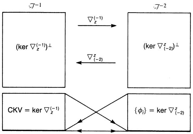
Figure 14.6. The map ${\nabla }_z^{(-)}$ and its adjoint ${\nabla }_{(-2)}^z$ .

$${\varphi }_{izz}\in \ker {\nabla }_{(-2)}^z.\text{\hspace{1em}(14.111)}$$

The explicit form of ${\nabla }_{(-2)}^z$ shows that ${\partial }_{\bar{z}}{\varphi }_{izz}=0$ , that is $\ker {\nabla }_{(-2)}^z$ is the set of holomorphic tensors of helicity $-2$ . The tensor ${\varphi }_i={\varphi }_{i\bar{z}z}\mathrm{d}z\otimes \mathrm{d}z$ is called the quadratic differential while ${\mu }_i={\mu }_{i\bar{z}z}\mathrm{d}z\otimes \mathrm{d}z$ is the Beltrami differential, see figure 14.7. In practical computations, it is often convenient to specify the gauge slice by the Beltrami differential, see later. Now we have established that

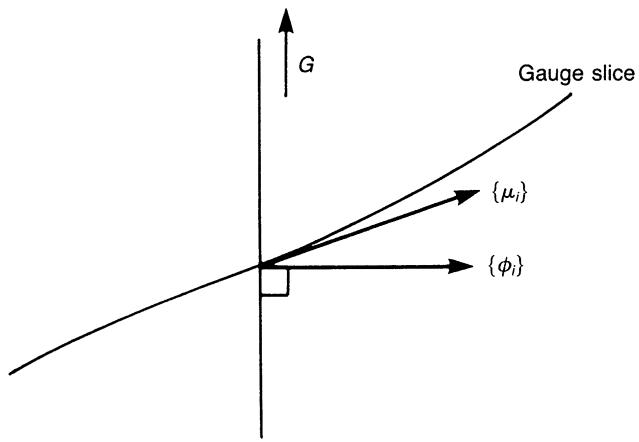
Figure 14.7. The Beltrami differential $\{{\mu }_i\}$ spans the deformation tangent to the gauge slice while $\{{\varphi }_i\}$ spans $\ker {\nabla }_{(-2)}^z$ .

$$\left\{\ker P_1^{†}\right\}=\left\{\text{Q u a d r a t i c d i f f e r e n t i a l}\right\}=\left\{\ker {\nabla }_{(-2)}^z\right\}.\text{\hspace{1em}(14.112)}$$

The Riemann-Roch theorem (14.27) takes the form

$${\dim }_{\mathbb{C}}\ker {\nabla }_z^{(-1)}-{\dim }_{\mathbb{C}}\ker {\nabla }_{(-2)}^z=3-3g.\text{\hspace{1em}(14.113)}$$

Now we have separated $\{\delta \gamma \}$ into mutually orthogonal pieces

$$\{\delta \gamma \}=\left\{\mathrm{conf}\right\}\oplus \left\{\mathrm{im}{\nabla }_z^{(-1)}\right\}\oplus \left\{\ker {\nabla }_{(-2)}^z\right\}+cc\text{\hspace{1em}(14.114)}$$

which should be compared with (14.80b). The measure becomes

$$\mathcal{D}\delta \gamma \mathcal{D}\delta X\to J{\mathrm{d}}^n\delta \tau \mathcal{D}\delta \bar{v}\mathcal{D}\delta \varphi \mathcal{D}\delta \tilde{X}{\mathrm{d}}^k\delta a\text{\hspace{1em}(14.115)}$$

where $n$ and $k$ are the complex dimensions of the Teichmüller space and the CKV, respectively. The Jacobian is obtained by repeating the argument in the previous subsection and we find that

$$\begin{array}{rl}{Z}_{\mathrm{g}}& =\int \mathcal{D}\gamma \mathcal{D}X\frac{1}{V(\text{D i f f}\ast \text{W e y l})}{\mathrm{e}}^{-S}\\ & ={\int }_{\text{M o d}}{\mathrm{d}}^n\tau \mathcal{D}X\frac{{\det }^{\prime }{\Delta }_{(1)}^{+}}{V(\mathrm{CKV})}\frac{|\det (\mu ,\varphi ){|}^2}{\det (\varphi ,\varphi )\det (\Phi ,\Phi )}{\mathrm{e}}^{-S}.\end{array}\text{\hspace{1em}(14.116)}$$

Since we are integrating over complex variables, the power of a half in (14.96)

does not appear in (14.116). The $X$ -integration yields

$$\begin{array}{rl}& Z_g={\int }_{\mathrm{Mod}}\frac{{\mathrm{d}}^n\tau }{V(\mathrm{CKV})}\frac{|\det (\mu ,\varphi ){|}^2}{\det (\varphi ,\varphi )\det (\Phi ,\Phi )}\\ & \times \stackrel{\prime }{\det }{\Delta }_{(1)}^{+}{\left(\frac{{\det }^{\prime }\Delta }{\int {\mathrm{d}}^{2}z\sqrt{\gamma }}\right)}^{-13}.\end{array}\text{\hspace{1em}(14.117)}$$

14.2.4 Moduli spaces of Riemann surfaces

The spaces $\mathrm{Mod}({\Sigma }_g)$ and Teich $({\Sigma }_g)$ have been defined as

$$\mathrm{Mod}\left({\Sigma }_{\mathrm{g}}\right)\equiv {\mathcal{M}}_g/\mathrm{Diff}\left({\Sigma }_{\mathrm{g}}\right)\mathrm{Teich}\left({\Sigma }_{\mathrm{g}}\right)\equiv {\mathcal{M}}_{\mathrm{g}}/{\mathrm{Diff}}_0\left({\Sigma }_{\mathrm{g}}\right).$$

They are related through MCG $\equiv$ $\mathrm{Diff}({\Sigma }_g)/{\mathrm{Diff}}_0({\Sigma }_g)$ as $\mathrm{Mod}({\Sigma }_g)=$ Teich $({\Sigma }_g)/\mathrm{MCG}$ . We look at these objects more closely here. We first note:

$$\begin{array}{ccccc}g& {\dim }_{\mathbb{C}}\mathrm{CKV}& \mathrm{CKV}& {\dim }_{\mathbb{C}}\mathrm{Teich}\left({\Sigma }_g\right)& \mathrm{MCG}\\ 0& 3& \mathrm{SL}(2,C)& 0& \mathrm{SL}(2,R)\\ 1& 1& \mathrm{U}(1)\times \mathrm{U}(1)& 1& \mathrm{SL}(2,Z)\\ \ge 2& 0& \text{e m p t y}& 3g-3& ?\end{array}\text{\hspace{1em}(14.118)}$$

[Remark: MCG for $g\ge 2$ can be expressed by $3g-1$ Dehn twists which are, however, not minimal.] From (14.118), we immediately conclude that $Z_0=0$ since the Teichmüller space is a single point and the volume of $\mathrm{SL}(2,\mathbb{C})$ is infinite. Of course, this does not imply that the three amplitudes with vertex operators vanish. In general, $\mathrm{Mod}({\Sigma }_g)$ is topologically non-trivial although $\mathrm{Teich}({\Sigma }_g)$ is. $\mathrm{Teich}({\Sigma }_g)$ is a universal covering space of $\mathrm{Mod}({\Sigma }_g)$ and the topological nontriviality comes from MCG.

In actual computations, the uniformization theorem is very useful. In the previous subsection, we first chose the Beltrami differential ${\mu }_i$ , then changed the basis to ${\varphi }_i\in \ker P_1^{†}$ . Our initial choice ${\mu }_i$ is motivated by the uniformization theorem.

Theorem 14.2 · Uniformization theorem

Let ${\Sigma }_g$ be a torus with genus $g$ . Then it is conformally related to the constant-curvature Riemann surface, which is given by the following:

where $L$ is a lattice in $\mathbb{C}$ (see example 8.2), $H$ the upper half-plane and $G\subset \mathrm{SL}(2,\mathbb{R})$ is called the Fuchsian group. The metric for $g\ge 2$ is the Poincaré metric, see example 7.6.

The proof of this theorem is found in Farkas and Kra (1980), for example. Thanks to this theorem, we may always take constant-curvature metrics to form the gauge slice in ${\mathcal{M}}_g$ . This corresponds to a special choice of the Beltrami differential ${\mu }_i$ . This slice defines the Weil-Petersson measure:

$$\int {\mathrm{d}}^n\tau \frac{{\left|\det (\mu ,\varphi )\right|}^2}{\det (\varphi ,\varphi )}=\int \mathrm{d}(\text{W e i l - P e t e r s s o n})\text{\hspace{1em}(14.120)}$$

see D’Hoker and Phong (1986).

Exercise 14.6

Compute the scalar curvature of the metrics given in (14.119). Verify that they are independent of $z$ and $\bar{z}$

Endnotes

Unplaced source note

Here $\ast$ denotes the semi-direct product. Note that $\mathrm{Diff}({\Sigma }_g)\cap \mathrm{Weyl}({\Sigma }_g)\ne \varnothing$ . We shall come back to this point later.

Unplaced source note

It should be kept in mind that we introduce the tangent space only to obtain the Jacobian. The tangent space itself has no physical relevance.

Unplaced source note

Since ${\psi }_0$ satisfies $\Delta {\psi }_0=0$ , it is a harmonic function. Any harmonic function on a Riemann surface must be a constant by the maximum principle.

Unplaced source note

In fact, the gauge is not uniquely fixed with this choice. We will invoke the uniformization theorem later to fix the gauge completely.

来源与版本

正文：英文 · OCR 机器稿 · 待校对

核对状态：OCR 机器稿 · 待校对

原书 PDF

来源版本：second-edition-local

来源 PDF SHA-256：fcd24c3371d092a8c699ccf5cf0765462924b6c48412804231076e8084b1940d

OCR 来源 SHA-256：0b6324f01172a3548cd34382e82fd8bfae574602b6b2cfaa357ba96bc2c35478

OCR 产物 SHA-256：1ece7cd9c3f57f1e59a74d4f3bb841b39a1734bcec13589b646e76b6c372b67f