3.1 The Metric

In Section 1, we informally introduced the metric as a way to measure distances between points. It does, indeed, provide this service but it is not its initial purpose. Instead, the metric is an inner product on each vector space $T_p(M)$

Definition

A metric g is a (0, 2) tensor field that is:

• Symmetric: $g(X,Y)=g(Y,X)$

• Non-Degenerate: If, for any $p\in M,g(X,Y){|}_p=0$ for all $Y\in T_p(M)$ then $X_p=0$ With a choice of coordinates, we can write the metric as

$$g=g_{\mu \nu }(x)d{x}^{\mu }\otimes d{x}^{\nu }$$

The object $g$ is often written as a line element $d{s}^2$ and this expression is abbreviated as

$$d{s}^2=g_{\mu \nu }(x)d{x}^{\mu }d{x}^{\nu }$$

This is the form that we saw previously in (1.4). The metric components can be extracted by evaluating the metric on a pair of basis elements,

$$g_{\mu \nu }(x)=g\left(\frac{\partial }{\partial x^{\mu }},\frac{\partial }{\partial x^{\nu }}\right)$$

The metric $g_{\mu \nu }$ is a symmetric matrix. We can always pick a basis $e_{\mu }$ of each $T_p(M)$ so that this matrix is diagonal. The non-degeneracy condition above ensures that none of these diagonal elements vanish. Some are positive, some are negative. Sylvester’s law of inertia is a theorem in algebra which states that the number of positive and negative entries is independent of the choice of basis. (This theorem has nothing to do with inertia. But Sylvester thought that if Newton could have a law of inertia, there should be no reason he couldn’t.) The number of negative entries is called the signature of the metric.

3.1.1 Riemannian Manifolds

For most applications of differential geometry, we are interested in manifolds in which all diagonal entries of the metric are positive. A manifold equipped with such a metric is called a Riemannian manifold. The simplest example is Euclidean space ${\mathbf{R}}^n$ which, in Cartesian coordinates, is equipped with the metric

$$g=d{x}^1\otimes d{x}^1+\dots +d{x}^n\otimes d{x}^n$$

The components of this metric are simply $g_{\mu \nu }={\delta }_{\mu \nu }$

A general Riemannian metric gives us a way to measure the length of a vector $X$ at each point,

$$|X|=\sqrt{g(X,X)}$$

It also allows us to measure the angle between any two vectors X and $Y$ at each point, using

$$g(X,Y)=|X||Y|\cos \theta$$

The metric also gives us a way to measure the distance between two points p and q along a curve in $M.$ . The curve is parameterised by $\sigma :[a,b]\to M$ , with $\sigma (a)=p$ and $\sigma (b)=q$ . The distance is then

$$\mathrm{distance}={\int }_a^{b}dt\sqrt{g(X,X){|}_{\sigma (t)}}$$

where X is a vector field that is tangent to the curve. If the curve has coordinates $x^{\mu }(t)$ , the tangent vector is $X^{\mu }=d{x}^{\mu }/dt$ , and the distance is

$$\mathrm{distance}={\int }_a^{b}dt\sqrt{g_{\mu \nu }(x)\frac{d{x}^{\mu }}{dt}\frac{d{x}^{\nu }}{dt}}$$

Importantly, this distance does not depend on the choice of parameterisation of the curve; this is essentially the same calculation that we did in Section 1.2 when showing the reparameterisation invariance of the action for a particle.

3.1.2 Lorentzian Manifolds

For the purposes of general relativity, we will be working with a manifold in which one of the diagonal entries of the metric is negative. A manifold equipped with such a metric is called Lorentzian.

The simplest example of a Lorentzian metric is Minkowski space. This is ${\mathbf{R}}^n$ equipped with the metric

$$\eta =-d{x}^0\otimes d{x}^0+d{x}^1\otimes d{x}^1+\cdots +d{x}^{n-1}\otimes d{x}^{n-1}$$

The components of the Minkowski metric are ${\eta }_{\mu \nu }=\mathrm{diag}(-1,+1,...,+1)$ . As this example shows, on a Lorentzian manifold we usually take the coordinate index $x^{\mu }$ to run from $0,1,\dots ,n-1$

At any point $p$ on a general Lorentzian manifold, it is always possible to find an orthonormal basis $\{e_{\mu }\}$ of $T_p(M)$ such that, locally, the metric looks like the Minkowski metric

$${g_{\mu \nu }|}_p={\eta }_{\mu \nu }\text{\hspace{1em}(3.1)}$$

This fact is closely related to the equivalence principle; we’ll describe the coordinates that allow us to do this in Section 3.3.2.

In fact, if we find one set of coordinates in which the metric looks like Minkowski space at $p,$ it is simple to exhibit other coordinates. Consider a different basis of vector fields related by

$${\tilde{e}}_{\mu }={\Lambda }_{\mu }^{\nu }{e}_{\nu }$$

Then, in this basis the components of the metric are

$${\tilde{g}}_{\mu \nu }={\Lambda }_{\mu }^{\rho }{\Lambda }_{\nu }^{\sigma }{g}_{\rho \sigma }$$

This leaves the metric in Minkowski form at p if

$${\eta }_{\mu \nu }={\Lambda }_{\mu }^{\rho }(p){\Lambda }_{\nu }^{\sigma }(p){\eta }_{\rho \sigma }\text{\hspace{1em}(3.2)}$$

This is the defining equation for a Lorentz transformation that we saw previously in (1.14). We see that viewed locally – which here means at a point $p-\mathrm{we}$ recover some basic features of special relativity. Note, however, that if we choose coordinates so that the metric takes the form (3.1) at some point $p,$ it will likely differ from the Minkowski metric as we move away from $p.$

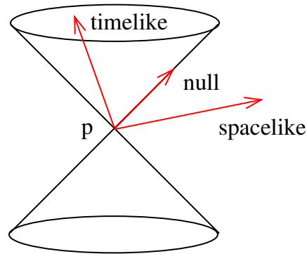
Figure 16. The lightcone at a point $p,$ with three different types of tangent vectors.

The fact that, locally, the metric looks like the Minkowski metric means that we can import some ideas from special relativity. At any point $p,$ a vector $X_p\in T_p(M)$ is said to be timelike if $g(X_p,X_p)<0$ , null if $g(X_p,X_p)=0$ , and spacelike if $g(X_p,X_p)>0$

At each point on M, we can then draw lightcones, which are the null tangent vectors at that point. There are both past-directed and future-directed lightcones at each point, as shown in Figure 16. The novelty is that the directions of these lightcones can vary smoothly as we move around the manifold. This specifies the causal structure of spacetime, which determines who can be friends with whom. We’ll see more of this later in the lectures.

We can again use the metric to determine the length of curves. The nature of a curve at a point is inherited from the nature of its tangent vector. A curve is called timelike if its tangent vector is everywhere timelike. In this case, we can again use the metric to measure the distance along the curve between two points $p$ and $q.$ Given a parametrisation $x^{\mu }(t)$ , this distance is,

$$\tau ={\int }_a^{b}dt\sqrt{-g_{\mu \nu }\frac{d{x}^{\mu }}{dt}\frac{d{x}^{\nu }}{dt}}$$

This is called the proper time. It is, in fact, something we’ve met before: it is precisely the action (1.27) for a point particle moving in the spacetime with metric $g_{\mu \nu }$

3.1.3 The Joys of a Metric

Whether we’re on a Riemannian or Lorentzian manifold, there are a number of bounties that the metric brings.

The Metric as an Isomorphism

First, the metric gives us a natural isomorphism between vectors and covectors, $g:$ $T_p(M)\to T_p^{\ast }(M)$ for each $p,$ with the one-form constructed from the contraction of $g$ and a vector field $X$

In a coordinate basis, we write $X=X^{\mu }{\partial }_{\mu }$ . This is mapped to a one-form which, because this is a natural isomorphism, we also call X. This notation is less annoying than you might think; in components the one-form is written is as $X=X_{\mu }d{x}^{\mu }$ . The components are then related by

$$X_{\mu }=g_{\mu \nu }{X}^{\nu }$$

Physicists usually say that we use the metric to lower the index from $X^{\mu }$ to $X_{\mu }$ . But in their heart, they mean “the metric provides a natural isomorphism between a vector space and its dual”.

Because g is non-degenerate, the matrix $g_{\mu \nu }$ is invertible. We denote the inverse as $g^{\mu \nu }$ , with $g^{\mu \nu }{g}_{\nu \rho }={\delta }_{\rho }^{\mu }$ . Here $g^{\mu \nu }$ can be thought of as the components of a symmetric (2, 0) tensor $\hat{g}=g^{\mu \nu }{\partial }_{\mu }\otimes {\partial }_{\nu }$ . More importantly, the inverse metric allows us to raise the index on a one-form to give us back the original tangent vector,

$$X^{\mu }=g^{\mu \nu }{X}_{\nu }$$

In Euclidean space, with Cartesian coordinates, the metric is simply $g_{\mu \nu }={\delta }_{\mu \nu }$ which is so simple it hides the distinction between vectors and one-forms. This is the reason we didn’t notice the difference between these spaces when we were five.

The Volume Form

The metric also gives us a natural volume form on the manifold M. On a Riemannian manifold, this is defined as

$$v=\sqrt{\det g_{\mu \nu }}d{x}^1\wedge \cdots \wedge d{x}^n$$

The determinant is usually simply written as $\sqrt{g}=\sqrt{\det g_{\mu \nu }}.$ . On a Lorentzian manifold, the determinant is negative and we instead have

$$v=\sqrt{-g}d{x}^0\wedge \cdots \wedge d{x}^{n-1}\text{\hspace{1em}(3.3)}$$

As defined, the volume form looks coordinate dependent. Importantly, it is not. To see this, introduce some rival coordinates ${\tilde{x}}^{\mu }$ , with

$$d{x}^{\mu }=A_{\nu }^{\mu }d{\tilde{x}}^{\nu }\text{ where }{A}_{\nu }^{\mu }=\frac{\partial x^{\mu }}{\partial {\tilde{x}}^{\nu }}$$

In the new coordinates, the wedgey part of the volume form becomes

$$d{x}^1\wedge \cdots \wedge d{x}^n=A_{{\mu }_1}^1\dots A_{{\mu }_n}^{n}d{\tilde{x}}^{{\mu }_1}\wedge \cdots \wedge d{\tilde{x}}^{{\mu }_n}$$

We can rearrange the one-forms into the order $d{\tilde{x}}^1$ $\wedge \dots \wedge d{\tilde{x}}^n$ . We pay a price of + $\mathrm{or}-1$ depending on whether $\{{\mu }_1,\dots ,{\mu }_n\}$ is an even or odd permutation of $\{1,\dots ,n\}$ Since we’re summing over all indices, this is the same as summing over all permutations π of $\{1,\dots ,n\}$ , and we have

$$\begin{array}{rl}d{x}^1\wedge \dots \wedge d{x}^n& =\sum _{\text{perms}\pi }\text{sign}(\pi )A_{\pi (1)}^1\dots A_{\pi (n)}^{n}d{\tilde{x}}^1\wedge \dots \wedge d{\tilde{x}}^n\\ & =\det (A)d{\tilde{x}}^1\wedge \dots \wedge d{\tilde{x}}^n\end{array}$$

where det $(A)>0$ if the change of coordinates preserves the orientation. This factor of $\det (A)$ is the usual Jacobian factor that one finds when changing the measure in an integral.

Meanwhile, the metric components transform as

$$g_{\mu \nu }=\frac{\partial {\tilde{x}}^{\rho }}{\partial x^{\mu }}\frac{\partial {\tilde{x}}^{\sigma }}{\partial x^{\nu }}{\tilde{g}}_{\rho \sigma }=(A^{-1}{)}_{\mu }^{\rho }(A^{-1}{)}_{\nu }^{\sigma }{\tilde{g}}_{\rho \sigma }$$

and so the determinant becomes

$$\det g_{\mu \nu }=(\det A^{-1}{)}^2\det {\tilde{g}}_{\mu \nu }=\frac{\det {\tilde{g}}_{\mu \nu }}{(\det A{)}^2}$$

We see that the factors of det A cancel, and we can equally write the volume form as

$$v=\sqrt{|\tilde{g}|}d{\tilde{x}}^1\wedge \cdots \wedge d{\tilde{x}}^n$$

The volume form (3.3) may look more familiar if we write it as

$$v=\frac{1}{n!}{v}_{{\mu }_1\dots {\mu }_n}d{x}^{{\mu }_1}\wedge \cdots \wedge d{x}^{{\mu }_n}$$

Here the components $v_{{\mu }_1\dots {\mu }_n}$ are given in terms of the totally anti-symmetric object ${ϵ}_{{\mu }_1\dots {\mu }_n}$ with ${ϵ}_{1\dots n}=+1$ and other components determined by the sign of the permutation,

$$v_{{\mu }_1\dots {\mu }_n}=\sqrt{|g|}{ϵ}_{{\mu }_1\dots {\mu }_n}\text{\hspace{1em}(3.4)}$$

Note that $v_{{\mu }_1\dots {\mu }_n}$ is a tensor, which means that ${ϵ}_{{\mu }_1\dots {\mu }_n}$ can’t quite be a tensor: instead, it is a tensor divided by $\sqrt{|g|}$ . It is sometimes said to be a tensor density. The antisymmetric tensor density arises in many places in physics. In all cases, it should be viewed as a volume form on the manifold. (In nearly all cases, this volume form arises from a metric as here.)

As with other tensors, we can use the metric to raise the indices and construct the volume form with all indices up

$$v^{{\mu }_1\dots {\mu }_n}=g^{{\mu }_1{\nu }_1}\dots g^{{\mu }_n{\nu }_n}{v}_{{\nu }_1\dots {\nu }_n}=\pm \frac{1}{\sqrt{|g|}}{ϵ}^{{\mu }_1\dots {\mu }_n}$$

where we get a + sign for a Riemannian manifold, and a − sign for a Lorentzian manifold. Here ${ϵ}^{{\mu }_1\dots {\mu }_n}$ is again a totally anti-symmetric tensor density with ${ϵ}^{\mathrm{1...}n}=+1$ Note, however, that while we raise the indices on $v_{{\mu }_1\dots {\mu }_n}$ using the metric, this statement doesn’t quite hold for ${ϵ}_{{\mu }_1\dots {\mu }_n}$ which takes values 1 or 0 regardless of whether the indices are all down or all up. This reflects the fact that it is a tensor density, rather than a genuine tensor.

The existence of a natural volume form means that, given a metric, we can integrate any function f over the manifold. We will sometimes write this as

$${\int }_{M}fv={\int }_M{d}^{n}x\sqrt{\pm g}f$$

The metric $\sqrt{\pm g}$ provides a measure on the manifold that tells us what regions of the manifold are weighted more strongly than the others in the integral.

The Hodge Dual

On an oriented manifold M, we can use the totally anti-symmetric tensor ${ϵ}_{{\mu }_1,\dots ,{\mu }_n}$ to define a map which takes a p-form $\omega \in {\Lambda }^p(M)$ to an $(n-p)$ -form, denoted $(\star \omega )\in$ ${\Lambda }^{n-p}(M)$ , defined by

$${\left(\star \omega \right)}_{{\mu }_1\dots {\mu }_{n-p}}=\frac{1}{p!}\sqrt{|g|}{ϵ}_{{\mu }_1\dots {\mu }_{n-p}{\nu }_1\dots {\nu }_p}{\omega }^{{\nu }_1\dots {\nu }_p}\text{\hspace{1em}(3.5)}$$

This map is called the Hodge dual. It is independent of the choice of coordinates.

It’s not hard to check that,

$$\star (\star \omega )=\pm (-1{)}^{p(n-p)}\omega \text{\hspace{1em}(3.6)}$$

where the + sign holds for Riemannian manifolds and the − sign for Lorentzian manifolds. (To prove this, it’s useful to first show that $v^{{\mu }_1...{\mu }_p{\rho }_1...{\rho }_{n-p}}{v}_{{\nu }_1...{\nu }_p{\rho }_1...{\rho }_{n-p}}=$ $\pm p!(n-p)!{\delta }_{[{\nu }_1}^{{\mu }_1}\cdot \cdot \cdot {\delta }_{{\nu }_p]}^{{\mu }_p}$ , again with the ± sign for Riemannian/Lorentzian manifolds.)

It’s worth returning to some high school physics and viewing it through the lens of our new tools. We are very used to taking two vectors in ${\mathbf{R}}^3$ , say a and b, and taking the cross-product to find a third vector

$$\mathbf{a}\times \mathbf{b}=\mathbf{c}$$

In fact, we really have objects that live in three different spaces here, related by the Euclidean metric ${\delta }_{\mu \nu }$ . First we use this metric to relate the vectors to one-forms. The cross-product is then really a wedge product which gives us back a 2-form. We then use the metric twice more, once to turn the two-form back into a one-form using the Hodge dual, and again to turn the one-form into a vector. Of course, none of these subtleties bothered us when we were 15. But when we start thinking about curved manifolds, with a non-trivial metric, these distinctions become important.

The Hodge dual allows us to define an inner product on each ${\Lambda }^p(M)$ . If ω, $\eta \in {\Lambda }^p(M)$ 2 we define

$$⟨\eta ,\omega ⟩={\int }_M\eta \wedge \star \omega$$

which makes sense because $\star \omega \in {\Lambda }^{n-p}(M)$ and so η $\wedge \star \omega$ is a top form that can be integrated over the manifold.

With such an inner product in place, we can also start to play the kind of games that are familiar from quantum mechanics and look at operators on ${\Lambda }^p(M)$ and their adjoints. The one operator that we have introduced on the space of forms is the exterior derivative, defined in Section 2.4.1. Its adjoint is defined by the following result:

Claim

For $\omega \in {\Lambda }^p(M)$ and $\alpha \in {\Lambda }^{p-1}(M)$

$$⟨d\alpha ,\omega ⟩=⟨\alpha ,d^{†}\omega ⟩\text{\hspace{1em}(3.7)}$$

where the adjoint operator $d^{†}:{\Lambda }^p(M)\to {\Lambda }^{p-1}(M)$ is given by

$$d^{†}=\pm (-1{)}^{np+n-1}\star d\star$$

with, again, the ± sign for Riemannian/Lorentzian manifolds respectively.

Proof

This is simply the statement of integration-by-parts for forms. On a closed manifold M, Stokes’ theorem tells us that

$$0={\int }_{M}d(\alpha \wedge \star \omega )={\int }_{M}d\alpha \wedge \star \omega +(-1{)}^{p-1}\alpha \wedge d\star \omega$$

The first term is simply $⟨d\alpha ,\omega ⟩$ . The second term also takes the form of an inner product which, up to a sign, is proportional to $⟨\alpha ,\star d\star \omega ⟩$ . To determine the sign, note that d $\star \omega \in {\Lambda }^{n-p+1}(M)$ so, using (3.6), we have ⋆ ⋆ d ⋆ $\omega =\pm (-1{)}^{(n-p+1)(p-1)}d\star \omega$ Putting this together gives

$$⟨d\alpha ,\omega ⟩=\pm (-1{)}^{np+n-1}⟨\alpha ,\star d\star \omega ⟩$$

as promised.

3.1.4 A Sniff of Hodge Theory

We can combine d and $d^{†}$ to construct the Laplacian, $△:{\Lambda }^p(M)\to {\Lambda }^p(M)$ , defined as

$$△=(d+d^{†}{)}^2=d{d}^{†}+d^{†}d$$

where the second equality follows because $d^2=d^{†2}=0$ . The Laplacian can be defined on both Riemannian manifolds, where it is positive definite, and Lorentzian manifolds. Here we restrict our discussion to Riemannian manifolds.

Acting on functions $f,$ we have $d^{†}$ $f=0$ (because $\star f$ is a top form so $d\star f=0)$ That leaves us with,

$$\begin{array}{rl}△(f)& =-\star d\star ({\partial }_{\mu }fd{x}^{\mu })\\ & =-\frac{1}{(n-1)!}\star d(({\partial }_{\mu }f)g^{\mu \nu }\sqrt{|g|}{ϵ}_{\nu {\rho }_1\dots {\rho }_{n-1}}d{x}^{{\rho }_1}\wedge \cdots \wedge d{x}^{{\rho }_{n-1}})\\ & =-\frac{1}{(n-1)!}\star {\partial }_{\sigma }(\sqrt{|g|}{g}^{\mu \nu }{\partial }_{\mu }f){ϵ}_{\nu {\rho }_1\dots {\rho }_{n-1}}d{x}^{\sigma }\wedge d{x}^{{\rho }_1}\wedge \cdots \wedge d{x}^{{\rho }_{n-1}}\\ & =-\star {\partial }_{\nu }(\sqrt{|g|}{g}^{\mu \nu }{\partial }_{\mu }f)d{x}^1\wedge \cdots \wedge d{x}^n\\ & =-\frac{1}{\sqrt{|g|}}{\partial }_{\nu }(\sqrt{|g|}{g}^{\mu \nu }{\partial }_{\mu }f)\end{array}$$

This form of the Laplacian, acting on functions, appears fairly often in applications of differential geometry.

There is a particularly nice story involving p-forms $\gamma$ that obey

$$△\gamma =0$$

Such forms are said to be harmonic. An harmonic form is necessarily closed, meaning $d\gamma =0$ , and co-closed, meaning $d^{†}\gamma =0$ . This follows by writing

$$⟨\gamma ,△\gamma ⟩=⟨d\gamma ,d\gamma ⟩+⟨d^{†}\gamma ,d^{†}\gamma ⟩=0$$

and noting that the inner product is positive-definite.

There are some rather pretty facts that relate the existence of harmonic forms to de Rham cohomology. The space of harmonic p-forms on a manifold M is denoted ${\mathrm{Harm}}^p(M)$ . First, the Hodge decomposition theorem, which we state without proof: any p-form ω on a compact, Riemannian manifold can be uniquely decomposed as

$$\omega =d\alpha +d^{†}\beta +\gamma$$

where $\alpha \in {\Lambda }^{p-1}(M)$ and $\beta \in {\Lambda }^{p+1}(M)$ and $\gamma \in {\mathrm{Harm}}^p(M)$ . This result can then be used to prove:

Hodge’s Theorem: There is an isomorphism

$${\mathrm{Harm}}^p(M)\cong H^p(M)$$

where $H^p(M)$ is the de Rham cohomology group introduced in Section 2.4.3. In particular, the Betti numbers can be computed by counting the number of linearly independent harmonic forms,

$$B_p=\dim {\mathrm{Harm}}^p(M)$$

Proof

First, let’s show that any harmonic form γ provides a representative of $H^p(M)$ As we saw above, any harmonic p-form is closed, $d\gamma =0$ , so $\gamma \in Z^p(M)$ . But the unique nature of the Hodge decomposition tells us that $\gamma \ne d\beta$ for some $\beta$

Next, we need to show that any equivalence class $[\omega ]\in H^p(M)$ can be represented by a harmonic form. We decompose $\omega =d\alpha +d^{†}\beta +\gamma$ . By definition $[\omega ]\in H^p(M)$ means that $d\omega =0$ so we have

$$0=⟨d\omega ,\beta ⟩=⟨\omega ,d^{†}\beta ⟩=⟨d\alpha +d^{†}\beta +\gamma ,d^{†}\beta ⟩=⟨d^{†}\beta ,d^{†}\beta ⟩$$

where, in the final step, we “integrated by parts” and used the fact that ddα $=d\gamma =0$ Because the inner product is positive definite, we must have $d^{†}\beta =0$ and, hence, $\omega =\gamma +d\alpha$ . Any other representative $\tilde{\omega }\sim \omega$ of $[\omega ]\in H^p(M)$ differs by $\tilde{\omega }=\omega +d\eta$ and so, by the Hodge decomposition, is associated to the same harmonic form $\gamma$ . □

来源与版本

正文：英文 · OCR 机器稿 · 待校对

核对状态：OCR 机器稿 · 待校对

原书 PDF

来源版本：michaelmas-2019-source-20260923

来源 PDF SHA-256：3ba65dc61f22a69c7d5fdf3e8e1f641efbfa6cf49a44b3dcb0fd5367ba9fcf1c

OCR 来源 SHA-256：4489f366864dc6e3f68337328d72571d937e8794fa6c9c377869436e2ed366c5

OCR 产物 SHA-256：9e61ec12e33054a372491e6319bd4cfc5bad4fa0169e3feb6d9a2c883d8ab59e