3.3 Parallel Transport

Although we have now met a number of properties of the connection, we have not yet explained its name. What does it connect?

The answer is that the connection connects tangent spaces, or more generally any tensor vector space, at different points of the manifold. This map is called parallel transport. As we stressed earlier, such a map is necessary to define differentiation.

Take a vector field X and consider some associated integral curve C, with coordinates $x^{\mu }(\tau )$ , such that

$$X^{\mu }{|}_C=\frac{d{x}^{\mu }(\tau )}{d\tau }\text{\hspace{1em}(3.25)}$$

We say that a tensor field T is parallely transported along C if

$${\nabla }_{X}T=0\text{\hspace{1em}(3.26)}$$

Suppose that the curve C connects two points, $p\in M$ and $q\in M$ . The requirement (3.26) provides a map from the vector space defined at p to the vector space defined at q.

To illustrate this, consider the parallel transport of a second vector field Y . In components, the condition (3.26) reads

$$X^{\nu }\left({\partial }_{\nu }{Y}^{\mu }+{\Gamma }_{\nu \rho }^{\mu }{Y}^{\rho }\right)=0$$

If we now evaluate this on the curve $C,$ we can think of $Y^{\mu }=Y^{\mu }(x(\tau ))$ , which obeys

$$\frac{d{Y}^{\mu }}{d\tau }+X^{\nu }{\Gamma }_{\nu \rho }^{\mu }{Y}^{\rho }=0\text{\hspace{1em}(3.27)}$$

These are a set of coupled, ordinary differential equations. Given an initial condition at, say $\tau =0$ , corresponding to point $p,$ these equations can be solved to find a unique vector at each point along the curve.

Parallel transport is path dependent. It depends on both the connection, and the underlying path which, in this case, is characterised by the vector field X.

This is the second time we’ve used a vector field X to construct maps between tensors at different points in the manifold. In Section 2.2.2, we used X to generate a flow ${\sigma }_t:M\to M$ , which we could then use to pull-back or push-forward tensors from one point to another. This was the basis of the Lie derivative. This is not the same as the present map. Here, we’re using X only to define the curve, while the connection does the work of relating vector spaces along the curve.

3.3.1 Geodesics Revisited

A geodesic is a curve tangent to a vector field X that obeys

$${\nabla }_{X}X=0\text{\hspace{1em}(3.28)}$$

Along the curve $C,$ we can substitute the expression (3.25) into (3.27) to find

$$\frac{d^2{x}^{\mu }}{d{\tau }^2}+{\Gamma }_{\rho \nu }^{\mu }\frac{d{x}^{\rho }}{d\tau }\frac{d{x}^{\nu }}{d\tau }=0\text{\hspace{1em}(3.29)}$$

This is precisely the geodesic equation (1.30) that we derived in Section 1 by considering the action for a particle moving in spacetime. In fact, we find that the condition (3.28) results in geodesics with affine parameterisation.

For the Levi-Civita connection, we have ${\nabla }_{X}g=0$ . This ensures that for any vector field Y parallely transported along a geodesic X, so ${\nabla }_{X}Y={\nabla }_{X}X=0$ , we have

$$\frac{d}{d\tau }g(X,Y)=0$$

This tells us that the vector field Y makes the same angle with the tangent vector along each point of the geodesic.

3.3.2 Normal Coordinates

Geodesics lend themselves to the construction of a particularly useful coordinate system. On a Riemannian manifold, in the neighbourhood of a point $p\in M$ , we can always find coordinates such that

$$g_{\mu \nu }(p)={\delta }_{\mu \nu }\mathrm{and}{g}_{\mu \nu ,\rho }(p)=0\text{\hspace{1em}(3.30)}$$

The same holds for Lorentzian manifolds, now with $g_{\mu \nu }(p)={\eta }_{\mu \nu }$ . These are referred to as normal coordinates. Because the first derivative of the metric vanishes, normal coordinates have the property that, at the point p, the Christoffel symbols vanish: ${\Gamma }_{\nu \rho }^{\mu }(p)=0$ . Generally, away from p we will have ${\Gamma }_{\nu \rho }^{\mu }\ne 0$ . Note, however, that it is not generally possible to ensure that the second derivatives of the metric also vanish. This, in turn, means that it’s not possible to pick coordinates such that the Riemann tensor vanishes at a given point.

There are a number of ways to demonstrate the existence of coordinates (3.30). The brute force way is to start with some metric ${\tilde{g}}_{\mu \nu }$ in coordinates ${\tilde{x}}^{\mu }$ and try to find a change of coordinates to $x^{\mu }(\tilde{x})$ which does the trick. In the new coordinates,

$$\frac{\partial {\tilde{x}}^{\rho }}{\partial x^{\mu }}\frac{\partial {\tilde{x}}^{\sigma }}{\partial x^{\nu }}{\tilde{g}}_{\rho \sigma }=g_{\mu \nu }\text{\hspace{1em}(3.31)}$$

We’ll take the point p to be the origin in both sets of coordinates. Then we can Taylor expand

$${\tilde{x}}^{\rho }={\frac{\partial {\tilde{x}}^{\rho }}{\partial x^{\mu }}|}_{x=0}{x}^{\mu }+\frac{1}{2}{\frac{{\partial }^2{\tilde{x}}^{\rho }}{\partial x^{\mu }\partial x^{\nu }}|}_{x=0}{x}^{\mu }{x}^{\nu }+\dots$$

We insert this into (3.31), together with a Taylor expansion of ${\tilde{g}}_{\rho \sigma }$ , and try to solve the resulting partial differential equations to find the coefficients $\partial \tilde{x}/\partial x$ and ${\partial }^2\tilde{x}/\partial x^2$ that do the job. For example, the first requirement is

$${\frac{\partial {\tilde{x}}^{\rho }}{\partial x^{\mu }}|}_{x=0}{\frac{\partial {\tilde{x}}^{\sigma }}{\partial x^{\nu }}|}_{x=0}{\tilde{g}}_{\rho \sigma }(p)={\delta }_{\mu \nu }$$

Given any ${\tilde{g}}_{\rho \sigma }(p)$ , it’s always possible to find $\partial \tilde{x}/\partial x$ so that this is satisfied. In fact, a little counting shows that there are many such choices. If dim $M=n$ , then there are $n^2$ independent coefficients in the matrix $\partial \tilde{x}/\partial x$ . The equation above puts $\frac{1}{2}n(n+1)$ conditions on these. That still leaves $\frac{1}{2}n(n-1)$ parameters unaccounted for. But this is to be expected: this is precisely the dimension of the rotational group $SO(n)$ (or the Lorentz group $SO(1,n-1))$ that leaves the flat metric unchanged.

We can do a similar counting at the next order. There are $\frac{1}{2}{n}^2(n+1)$ independent elements in the coefficients ${\partial }^2{\tilde{x}}^{\rho }/\partial x^{\mu }\partial x^{\nu }$ . This is exactly the same number of conditions in the requirement $g_{\mu \nu ,\rho }(p)=0$

We can also see why we shouldn’t expect to set the second derivative of the metric to zero. Requiring $g_{\mu \nu ,\rho \sigma }=0$ is $\frac{1}{4}{n}^2(n+1{)}^2$ constraints. Meanwhile, the next term in the Taylor expansion is ${\partial }^3{\tilde{x}}^{\rho }/\partial x^{\mu }\partial x^{\nu }\partial x^{\lambda }$ which has $\frac{1}{6}{n}^2(n+1)(n+2)$ independent coefficients. We see that the numbers no longer match. This time we fall short, leaving

$$\frac{1}{4}{n}^2(n+1{)}^2-\frac{1}{6}{n}^2(n+1)(n+2)=\frac{1}{12}{n}^2(n^2-1)$$

unaccounted for. This, therefore, is the number of ways to characterise the second derivative of the metric in a manner that cannot be undone by coordinate transformations. Indeed, it is not hard to show that this is precisely the number of independent coefficients in the Riemann tensor. (For $n=4$ n = 4 , there are 20 coefficients of the Riemann tensor.)

The Exponential Map

There is a rather pretty, direct way to construct the coordinates (3.30). This uses geodesics. The rough idea is that, given a tangent vector $X_p\in T_p(M)$ , there is a unique affinely parameterised geodesic through p with tangent vector $X_p$ at $p.$ . We then label any point $q$ in the neighbourhood of $p$ by the coordinates of the geodesic that take us to $q$ in some fixed amount of time. It’s like throwing a ball in all possible directions, and labelling points by the initial velocity needed for the ball to reach that point in, say, 1 second.

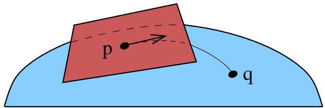
Figure 17. Start with a tangent vector, and follow the resulting geodesic to get the exponential map.

Let’s put some flesh on this. We introduce any coordinate system (not necessarily normal coordinates) ${\tilde{x}}^{\mu }$ in the neighbourhood of $p.$ . Then the geodesic we want solves the equation (3.29) subject to the requirements

$${\frac{d{\tilde{x}}^{\mu }}{d\tau }|}_{\tau =0}={\tilde{X}}_p^{\mu }\mathrm{with}{\tilde{x}}^{\mu }(\tau =0)=0$$

There is a unique solution.

This observation means that we can define a map,

$$\mathrm{Exp}:T_p(M)\to M$$

Given $X_p\in T_p(M)$ , construct the appropriate geodesic and the follow it for some affine distance which we take to be $\tau =1$ . This gives a point $q\in M$ . This is known as the exponential map and is illustrated in the Figure 17.

There is no reason that the exponential map covers all of the manifold M. It could well be that there are points which cannot be reached from $p$ by geodesics. Moreover, it may be that there are tangent vectors $X_p$ for which the exponential map is ill-defined. In general relativity, this occurs if the spacetime has singularities. Neither of these issues are relevant for our current purpose.

Now pick a basis $\{e_{\mu }\}$ of $T_p(M)$ . The exponential map means that tangent vector $X_p=X^{\mu }{e}_{\mu }$ defines a point $q$ in the neighbourhood of $p.$ We simply assign this point coordinates

$$x^{\mu }(q)=X^{\mu }$$

These are the normal coordinates.

If we pick the initial basis $\{e_{\mu }\}$ to be orthonormal, then the geodesics will point in orthogonal directions which ensures that the metric takes the form $g_{\mu \nu }(p)={\delta }_{\mu \nu }$

To see that the first derivative of the metric also vanishes, we first fix a point q associated to a given tangent vector $X\in T_p(M)$ . This tells us that the point q sits a distance $\tau =1$ along the geodesic. We can now ask: what tangent vector will take us a different distance along this same geodesic? Because the geodesic equation (3.29) is homogeneous in $\tau ,$ if we halve the length of X then we will travel only half the distance along the geodesic, i.e. to $\tau =1/2$ . In general, the tangent vector $\tau X$ will take us a distance $\tau$ along the geodesic

$$\mathrm{Exp}:\tau X_p\to x^{\mu }(\tau )=\tau X^{\mu }$$

This means that the geodesics in these coordinates take the particularly simply form

$$x^{\mu }(\tau )=\tau X^{\mu }$$

Since these are geodesics, they must solve the geodesic equation (3.29). But, for trajectories that vary linearly in time, this is just

$${\Gamma }_{\rho \nu }^{\mu }(x(\tau ))X^{\rho }{X}^{\nu }=0$$

This holds at any point along the geodesic. At most points $x(\tau )$ , this equation only holds for those choices of $X^{\rho }$ which take us along the geodesic in the first place. However, at $x(\tau )=0$ , corresponding to the point $p$ of interest, this equation must hold for any tangent vector $X^{\mu }$ . This means that ${\Gamma }_{(\rho \nu )}^{\mu }(p)=0$ which, for a torsion free connection, ensures that ${\Gamma }_{\rho \nu }^{\mu }(p)=0$

Vanishing Christoffel symbols means that the derivative of the metric vanishes. This follows for the Levi-Civita connection by writing $2g_{\mu \sigma }{\Gamma }_{\rho \nu }^{\sigma }=g_{\mu \rho ,\nu }+g_{\mu \nu ,\rho }-g_{\rho \nu ,\mu }.$ Symmetrising over $(\mu \rho )$ means that the last two terms cancel, leaving us with $g_{\mu \rho ,\nu }=0$ when evaluated at $p.$

The Equivalence Principle

Normal coordinates play an important conceptual role in general relativity. Any observer at point $p$ who parameterises her immediate surroundings using coordinates constructed by geodesics will experience a locally flat metric, in the sense of (3.30).

This is the mathematics underlying the Einstein equivalence principle. This principle states that any freely falling observer, performing local experiments, will not experience a gravitational field. Here “freely falling” means the observer follows geodesics, as we saw in Section 1 and will naturally use normal coordinates. In this context, the coordinates are called a local inertial frame. The lack of gravitational field is the statement that $g_{\mu \nu }(p)={\eta }_{\mu \nu }$

Key to understanding the meaning and limitations of the equivalence principle is the word “local”. There is a way to distinguish whether there is a gravitational field at $p:$ we compute the Riemann tensor. This depends on the second derivative of the metric and, in general, will be non-vanishing. However, to measure the effects of the Riemann tensor, one typically has to compare the result of an experiment at $p$ with an experiment at a nearby point $q:$ this is considered a “non-local” observation as far as the equivalence principle goes. In the next two subsections, we give examples of physics that depends on the Riemann tensor.

3.3.3 Path Dependence: Curvature and Torsion

Take a tangent vector $Z_p\in T_p(M)$ , and parallel transport it along a curve $C$ to some point $r\in M$ . Now parallel transport it along a different curve $C^{\prime }$ to the same point $r.$ . How do the resulting vectors differ?

To answer this, we construct each of our curves C and $C^{\prime }$ from two segments, generated by linearly independent vector fields, X and Y satisfying $[X,Y]=0$ as shown in Figure 18. To make life easy, we’ll take the point r to be close to the original point $p.$

We pick normal coordinates $x^{\mu }=(\tau ,\sigma ,0,\dots )$ so that the starting point is at $x^{\mu }(p)=0$ while the tangent vectors are aligned along the coordinates, $X=\partial /\partial \tau$ and $Y=\partial /\partial \sigma$ The other corner points are then $x^{\mu }(q)=(\delta \tau ,0,0,...),x^{\mu }(r)=(\delta \tau ,\delta \sigma ,0,...)$ and $x^{\mu }(s)=(0,\delta \sigma ,0,...)$ where $\delta \tau$ and δσ are taken to be small. This set-up is shown in Figure 18.

First we parallel transport $Z_p$ along X to $Z_q$ . Along the curve, $Z^{\mu }$ solves (3.27)

$$\frac{d{Z}^{\mu }}{d\tau }+X^{\nu }{\Gamma }_{\rho \nu }^{\mu }{Z}^{\rho }=0\text{\hspace{1em}(3.32)}$$

We Taylor expand the solution as

$$Z_q^{\mu }=Z_p^{\mu }+{\frac{d{Z}^{\mu }}{d\tau }|}_{\tau =0}\delta \tau +\frac{1}{2}{\frac{d^2{Z}^{\mu }}{d{\tau }^2}|}_{\tau =0}\delta {\tau }^2+\mathcal{O}(\delta {\tau }^3)$$

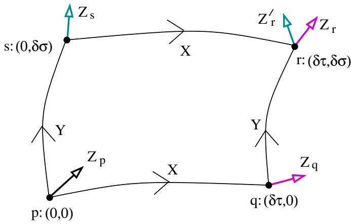
Figure 18. Parallel transporting a vector $Z_p$ along two different paths does not give the same answer.

From (3.32), we have $d{Z}^{\mu }/d\tau {|}_0=0$ because, in normal coordinates, ${\Gamma }^{\mu }{}_{\rho \nu }(p)=0$ . We can calculate the second derivative by differentiating (3.32) to find

$$\begin{array}{rl}& {\frac{d^2{Z}^{\mu }}{d{\tau }^2}|}_{\tau =0}=-\left(X^{\nu }{Z}^{\rho }\frac{d{\Gamma }_{\rho \nu }^{\mu }}{d\tau }+\frac{d{X}^{\nu }}{d\tau }{Z}^{\rho }{\Gamma }_{\rho \nu }^{\mu }+X^{\nu }\frac{d{Z}^{\rho }}{d\tau }{\Gamma }_{\rho \nu }^{\mu }\right){|}_p\\ & =-{X^{\nu }{Z}^{\rho }\frac{d{\Gamma }_{\rho \nu }^{\mu }}{d\tau }|}_p\\ & =-(X^{\nu }{X}^{\sigma }{Z}^{\rho }{\Gamma }_{\rho \nu ,\sigma }^{\mu }{)}_p\end{array}\text{\hspace{1em}(3.33)}$$

Here the second line follows because we’re working in normal coordinates at $p,$ and the final line because $\tau$ is the parameter along the integral curve of $X$ , so $d/d\tau =X^{\sigma }{\partial }_{\sigma }$ We therefore have

$$Z_q^{\mu }=Z_p^{\mu }-\frac{1}{2}(X^{\nu }{X}^{\sigma }{Z}^{\rho }{\Gamma }_{\rho \nu ,\sigma }^{\mu }{)}_p\delta {\tau }^2+\dots \text{\hspace{1em}(3.34)}$$

Now we parallel transport once more, this time along $Y$ to $Z_r^{\mu }$ . The Taylor expansion now takes the form

$$Z_r^{\mu }=Z_q^{\mu }+{\frac{d{Z}^{\mu }}{d\sigma }|}_q\delta \sigma +\frac{1}{2}{\frac{d^2{Z}^{\mu }}{d{\sigma }^2}|}_q\delta {\sigma }^2+\mathcal{O}(\delta {\sigma }^3)\text{\hspace{1em}(3.35)}$$

We can again evaluate the first derivative $d{Z}^{\mu }/d\sigma {|}_q$ using the analog of the parallel transport equation (3.32),

$${\frac{d{Z}^{\mu }}{d\sigma }|}_q=-(Y^{\nu }{Z}^{\rho }{\Gamma }_{\rho \nu }^{\mu }{)}_q$$

Since we’re working in normal coordinates about $p$ and not $q,$ we no longer get to argue that this term vanishes. Instead we Taylor expand about $p$ to get

$$(Y^{\nu }{Z}^{\rho }{\Gamma }_{\rho \nu }^{\mu }{)}_q=(Y^{\nu }{Z}^{\rho }{X}^{\sigma }{\Gamma }_{\rho \nu ,\sigma }^{\mu }{)}_p\delta \tau +\dots$$

Note that in principle we should also Taylor expand $Y^{\nu }$ and $Z^{\rho }$ but, at leading order, these will multiply ${\Gamma }_{\rho \nu }^{\mu }(p)=0$ , so they only contribute at next order. The second order term in the Taylor expansion (3.35) involves $d^2{Z}^{\mu }/d{\sigma }^2{|}_q$ and there is an expression similar to (3.33). To leading order the $d{X}^{\nu }/d\sigma$ and $d{Z}^{\rho }/d\sigma$ terms are again absent because they are multiplied by ${\Gamma }_{\rho \nu }^{\mu }(q)=d{\Gamma }_{\rho \nu }^{\mu }/d\tau {|}_p\delta \tau$ . We therefore have

$$\begin{array}{rl}& \frac{d^2{Z}^{\mu }}{d{\sigma }^2}{|}_q=-(Y^{\nu }{Y}^{\sigma }{Z}^{\rho }{\Gamma }_{\rho \nu ,\sigma }^{\mu }{)}_q+\dots \\ & =-(Y^{\nu }{Y}^{\sigma }{Z}^{\rho }{\Gamma }_{\rho \nu ,\sigma }^{\mu }{)}_p+\dots \end{array}$$

where we replaced the point q with point p because they differ only subleading terms proportional to $\delta \tau$ . The upshot is that this time the difference between $Z_r^{\mu }$ and $Z_q^{\mu }$ involves two terms,

$$Z_r^{\mu }=Z_q^{\mu }-(Y^{\nu }{Z}^{\rho }{X}^{\sigma }{\Gamma }_{\rho \nu ,\sigma }^{\mu }{)}_p\delta \tau \delta \sigma -\frac{1}{2}(Y^{\nu }{Y}^{\sigma }{Z}^{\rho }{\Gamma }_{\rho \nu ,\sigma }^{\mu }{)}_p\delta {\sigma }^2+\dots$$

Finally, we can relate $Z_q^{\mu }$ to $Z_p^{\mu }$ using the expression (3.34) that we derived previously. We end up with

$$Z_r^{\mu }=Z_p^{\mu }-\frac{1}{2}({\Gamma }_{\rho \nu ,\sigma }^{\mu }{)}_p{\left[X^{\nu }{X}^{\sigma }{Z}^{\rho }\delta {\tau }^2+2Y^{\nu }{Z}^{\rho }{X}^{\sigma }\delta \sigma \delta \tau +Y^{\nu }{Y}^{\sigma }{Z}^{\rho }\delta {\sigma }^2\right]}_p+\dots$$

where … denotes any terms cubic or higher in small quantities.

Now suppose we go along the path $C^{\prime },$ first visiting point s and then making our way to r. We can read the answer of directly from the result above, simply by swapping X and Y and $\sigma$ and $\tau ;$ only the middle term changes,

$$Z_r^{\prime \mu }=Z_p^{\mu }-\frac{1}{2}({\Gamma }_{\rho \nu ,\sigma }^{\mu }{)}_p{\left[X^{\nu }{X}^{\sigma }{Z}^{\rho }\delta {\tau }^2+2X^{\nu }{Z}^{\rho }{Y}^{\sigma }\delta \sigma \delta \tau +Y^{\nu }{Y}^{\sigma }{Z}^{\rho }\delta {\sigma }^2\right]}_p+\dots$$

We find that

$$\begin{array}{rl}& \Delta Z_r^{\mu }=Z_r^{\mu }-Z_r^{\prime \mu }=-({\Gamma }_{\rho \nu ,\sigma }^{\mu }-{\Gamma }_{\rho \sigma ,\nu }^{\mu }{)}_p(Y^{\nu }{Z}^{\rho }{X}^{\sigma }{)}_p\delta \sigma \delta \tau +\dots \\ & =(R_{\rho \sigma \nu }^{\mu }{Y}^{\nu }{Z}^{\rho }{X}^{\sigma }{)}_p\delta \sigma \delta \tau +\dots \end{array}$$

where, in the final equality, we’ve used the expression for the Riemann tensor in components (3.15), which simplifies in normal coordinates as ${\Gamma }_{\rho \sigma }^{\mu }(p)=0$ . Note that, to the order we’re working, we could equally as well evaluate $R^{\mu }{}_{\rho \sigma \nu }{X}^{\nu }{Z}^{\rho }{Y}^{\sigma }$ at the point $r;$ the two differ only by higher order terms.

Although our calculation was performed with a particular choice of coordinates, the end result is written as an equality between tensors and must, therefore, hold in any coordinate system. This is a trick that we will use frequently throughout these lectures: calculations are considerably easier in normal coordinates. But if the resulting expression relate tensors then the final result must be true in any coordinate system.

We have discovered a rather nice interpretation of the Riemann tensor: it tells us the path dependence of parallel transport. The calculation above is closely related to the idea of holonomy. Here, one transports a vector around a closed curve C and asks how the resulting vector compares to the original. This too is captured by the Riemann tensor. A particularly simple example of non-trivial holonomy comes from parallel transport of a vector on a sphere: the direction that you end up pointing in depends on the path you take.

The Meaning of Torsion

We discarded torsion almost as soon as we met it, choosing to work with the Levi-Civita connection which has vanishing torsion, ${\Gamma }_{\mu \nu }^{\rho }={\Gamma }_{\nu \mu }^{\rho }$ . Moreover, as we will see in Section 4, torsion plays no role in the theory of general relativity which makes use of the Levi-Civita connection. Nonetheless, it is natural to ask: what is the geometric meaning of torsion? There is an answer to this that makes use of the kind of parallel transport arguments we used above.

This time, we start with two vectors $X,Y\in$ $T_p(M)$ . We pick coordinates $x^{\mu }$ and write these vectors as $X=X^{\mu }{\partial }_{\mu }$ and $Y=Y^{\mu }{\partial }_{\mu }$ . Starting from $p\in M$ , we can use these two vectors to construct two points infinitesimally close to $p.$ We call these points r and s respectively: they have coordinates

$$r:x^{\mu }+X^{\mu }ϵ\mathrm{and}s:x^{\mu }+Y^{\mu }ϵ$$

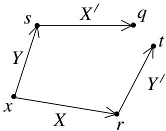
where ϵ is some infinitesimal parameter.

We now parallel transport the vector $X\in T_p(M)$ along the direction of $Y$ to give a new vector $X^{\prime }\in T_s(M)$ . Similarly, we parallel transport Y along the direction of X to get a new vector $Y^{\prime }\in T_r(M)$ . These new vectors have components

$$X^{\prime }=(X^{\mu }-ϵ{\Gamma }_{\nu \rho }^{\mu }{Y}^{\nu }{X}^{\rho }){\partial }_{\mu }\mathrm{and}{Y}^{\prime }=(Y^{\mu }-ϵ{\Gamma }_{\nu \rho }^{\mu }{X}^{\nu }{Y}^{\rho }){\partial }_{\mu }$$

Each of these tangent vectors now defines a new point. Starting from point s, and moving in the direction of $X^{\prime }$ , we see that we get a new point $q$ with coordinates

$$q:x^{\mu }+(X^{\mu }+Y^{\mu })ϵ-{ϵ}^2{\Gamma }_{\nu \rho }^{\mu }{Y}^{\nu }{X}^{\rho }$$

Meanwhile, if we sit at point r and move in the direction of $Y^{\prime }$ , we get to a typically different point, $t,$ with coordinates

$$t:x^{\mu }+(X^{\mu }+Y^{\mu })ϵ-{ϵ}^2{\Gamma }_{\nu \rho }^{\mu }{X}^{\nu }{Y}^{\rho }$$

We see that if the connection has torsion, so ${\Gamma }_{\nu \rho }^{\mu }\ne {\Gamma }_{\rho \nu }^{\mu }.$ , then the two points $q$ and t do not coincide. In other words, torsion measures the failure of the parallelogram shown in figure to close.

3.3.4 Geodesic Deviation

Consider now a one-parameter family of geodesics, with coordinates $x^{\mu }(\tau ;s)$ . Here $\tau$ is the affine parameter along the geodesics, all of which are tangent to the vector field X so that, along the surface spanned by $x^{\mu }(\tau ,s)$ , we have

$$X^{\mu }={\frac{\partial x^{\mu }}{\partial \tau }|}_s$$

Meanwhile, s labels the different geodesics, as shown in Figure 19. We take the tangent vector in the s direction to be generated by a second vector field S so that,

$$S^{\mu }={\frac{\partial x^{\mu }}{\partial s}|}_{\tau }$$

The tangent vector $S^{\mu }$ is sometimes called the deviation vector; it takes us from one geodesic to a nearby geodesic with the same affine parameter $\tau .$

The family of geodesics sweeps out a surface embedded in the manifold. This gives us some freedom in the way we assign coordinates s and τ. In fact, we can always pick coordinates s and t on the surface such that $S=\partial /\partial s$ and $X=\partial /\partial t$ , ensuring that

$$[S,X]=0$$

Roughly speaking, we can do this if we use τ and s as coordinates on some submanifold of M. Then the vector fields can be written simply as $X=\partial /\partial \tau$ and $S=\partial /\partial s$ and $[X,S]=0$

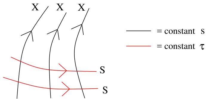
Figure 19. The black lines are geodesics generated by X. The red lines label constant τ and are generated by S, with $[X,S]=0$

We can ask how neighbouring geodesics behave. Do they converge? Or do they move further apart? Now consider a connection Γ with vanishing torsion, so that ${\nabla }_{X}S-{\nabla }_{S}X=[X,S]$ . Since $[X,S]=0$ , we have

$${\nabla }_X{\nabla }_{X}S={\nabla }_X{\nabla }_{S}X={\nabla }_S{\nabla }_{X}X+R(X,S)X$$

where, in the second equality, we’ve used the expression (3.14) for the Riemann tensor as a differential operator. But ${\nabla }_{X}X=0$ because X is tangent to geodesics, and we have

$${\nabla }_X{\nabla }_{X}S=R(X,S)X$$

In index notation, this is

$$X^{\nu }{\nabla }_{\nu }(X^{\rho }{\nabla }_{\rho }{S}^{\mu })=R_{\nu \rho \sigma }^{\mu }{X}^{\nu }{X}^{\rho }{S}^{\sigma }$$

If we further restrict to an integral curve C associated to the vector field $X$ , as in (3.25), this equation is sometimes written as

$$\frac{D^2{S}^{\mu }}{D{\tau }^2}=R_{\nu \rho \sigma }^{\mu }{X}^{\nu }{X}^{\rho }{S}^{\sigma }\text{\hspace{1em}(3.36)}$$

where $D/D\tau$ is the covariant derivative along the curve $C,$ defined by $\begin{array}{r}D/D\tau =\frac{\partial x^{\mu }}{\partial \tau }{\nabla }_{\mu }\end{array}$ The left-hand-side tells us how the deviation vector $S^{\mu }$ changes as we move along the geodesic. In other words, it is the relative acceleration of neighbouring geodesics. We learn that this relative acceleration is controlled by the Riemann tensor.

Experimentally, such geodesic deviations are called tidal forces. We met a simple example in Section 1.2.4.

An Example: the Sphere ${\mathbf{S}}^2$ Again

It is simple to determine the geodesics on the sphere ${\mathbf{S}}^2$ of radius r. Using the Christoffel symbols (3.19), the geodesic equations are

$$\frac{d^2\theta }{d{\tau }^2}=\sin \theta \cos \theta {\left(\frac{d\varphi }{d\tau }\right)}^2\mathrm{and}\frac{d^2\varphi }{d{\tau }^2}=-2\frac{\cos \theta }{\sin \theta }\frac{d\varphi }{d\tau }\frac{d\theta }{d\tau }$$

The solutions are great circles. The general solution is a little awkward in these coordinates, but there are two simple solutions.

• We can set $\theta =\pi /2$ with $\dot{\theta }=0$ and $\dot{\varphi }=\mathrm{constant}$ . This is a solution in which the particle moves around the equator. Note that this solution doesn’t work for other values of θ.

• We can set $\dot{\varphi }=0$ and $\dot{\theta }=\mathrm{constant}$ . These are paths of constant longitude and are geodesics for any constant value of $\varphi .$ . Note, however, that our coordinates go a little screwy at the poles $\theta =0$ and $\theta =\pi$

To illustrate geodesic deviation, we’ll look at the second class of solutions; the particle moves along $\theta =v\tau$ , with the angle $\varphi$ specifying the geodesic. This set-up is simple enough that we don’t need to use any fancy Riemann tensor techniques: we can just understand the geodesic deviation using simple geometry. The distance between the geodesic at $\varphi =0$ and the geodesic at some other longitude $\varphi$ is

$$s(\tau )=r\varphi \sin \theta =r\varphi \sin (v\tau )\text{\hspace{1em}(3.37)}$$

Now let’s re-derive this result using our fancy technology. The geodesics are generated by the vector field $X^{\theta }=v$ . Meanwhile, the separation between geodesics at a fixed $\tau$ is $S^{\varphi }=s(\tau )$ . The geodesic deviation equation in the form (3.36) is

$$\frac{d^{2}s}{d{\tau }^2}=v^2{R}_{\theta \theta \varphi }^{\varphi }s(\tau )$$

We computed the Riemann tensor for ${\mathbf{S}}^2$ in (3.20); the relevant component is

$$R_{\varphi \theta \theta \varphi }=-r^2{\sin }^2\theta \Rightarrow R_{\theta \theta \varphi }^{\varphi }=g^{\varphi \varphi }{R}_{\varphi \theta \theta \varphi }=-1\text{\hspace{1em}(3.38)}$$

and the geodesic deviation equation becomes simply

$$\frac{d^{2}s}{d{\tau }^2}=-v^{2}s$$

which is indeed solved by (3.37).

来源与版本

正文：英文 · OCR 机器稿 · 待校对

核对状态：OCR 机器稿 · 待校对

原书 PDF

来源版本：michaelmas-2019-source-20260923

来源 PDF SHA-256：3ba65dc61f22a69c7d5fdf3e8e1f641efbfa6cf49a44b3dcb0fd5367ba9fcf1c

OCR 来源 SHA-256：4489f366864dc6e3f68337328d72571d937e8794fa6c9c377869436e2ed366c5

OCR 产物 SHA-256：fc3ec63aecaa3cd2f1c5ef1e64a4a2047bc93b1cccc3a2cae790389edb1d138f