4.2 Some Simple Solutions

We will now look for some simple solutions to the Einstein equations

$$R_{\mu \nu }=\Lambda g_{\mu \nu }$$

As we will see, the solutions take a very different form depending on whether Λ is zero, positive or negative.

Minkowski Space

Let’s start with $\Lambda =0$ . Here the vacuum Einstein equations reduce to $R_{\mu \nu }=0$ . If we’re looking for the simplest solution to this equation, it’s tempting to suggest $g_{\mu \nu }=0$ Needless to say, this isn’t allowed! The tensor field $g_{\mu \nu }$ is a metric and, as defined in Section 3, must be non-degenerate. Indeed, the existence of the inverse $g^{\mu \nu }$ was assumed in the derivation of the Einstein equations from the action.

While this restriction is natural geometrically, it is rather unusual from the perspective of a physical theory. It is not a holonomic constraint on the physical degrees of freedom: instead it is an inequality det $g_{\mu \nu }<0$ (together with the requirement that $g_{\mu \nu }$ has one, rather than three, negative eigenvalues). Other fields in the Standard Model don’t come with such restrictions. Instead, it is reminiscent of fluid mechanics where one has to insist that matter density obeys $\rho (\mathbf{x},t)>0$ . Ultimately, it seems likely that this restriction is telling us that the gravitational field is not fundamental and should be replaced by something else in regimes where det $g_{\mu \nu }$ is getting small.

The restriction that det $g_{\mu \nu }\ne 0$ means that the simplest Ricci flat metric is Minkowski space, with

$$d{s}^2=-d{t}^2+d{\mathbf{x}}^2$$

Of course, this is far from the only metric obeying $R_{\mu \nu }=0$ . Another example is provided by the Schwarzschild metric,

$$d{s}^2=-\left(1-\frac{2GM}{r}\right)d{t}^2+{\left(1-\frac{2GM}{r}\right)}^{-1}d{r}^2+r^2(d{\theta }^2+{\sin }^2\theta d{\varphi }^2)\text{\hspace{1em}(4.8)}$$

which we will discuss further in Section 6. We will meet more solutions as the course progresses.

4.2.1 de Sitter Space

We now turn to the Einstein equations with $\Lambda >0$ . Once again, there are many solutions. Since it’s a pain to solve the Einstein equations, let’s work with an ansatz that we’ve already seen. Suppose that we look for solutions of the form

$$d{s}^2=-f(r{)}^{2}d{t}^2+f(r{)}^{-2}d{r}^2+r^2(d{\theta }^2+{\sin }^2\theta d{\varphi }^2)\text{\hspace{1em}(4.9)}$$

We already computed the components of the Riemann tensor for such a metric in Section 3.4.3 using the technology of curvature 2-forms. From the result, given in (3.54), we can easily check that the Ricci tensor is diagonal with components

$$R_{tt}=-f^4{R}_{rr}=f^3\left(f^{\prime \prime }+\frac{2f^{\prime }}{r}+\frac{f^{\prime 2}}{f}\right)$$

and

$$R_{\varphi \varphi }={\sin }^2\theta R_{\theta \theta }=(1-f^2-2f{f}^{\prime }r){\sin }^2\theta$$

The resulting Ricci tensor can indeed be made to be proportional to the metric, with $R_{\mu \nu }=\Lambda g_{\mu \nu }$ . Comparing to (4.9), we see that the function $f(r)$ must satisfy two constraints. The first comes from the tt and rr components,

$$f^{\prime \prime }+\frac{2f^{\prime }}{r}+\frac{f^2}{f}=-\frac{\Lambda }{f}\text{\hspace{1em}(4.10)}$$

The second comes from the θθ and $\varphi \varphi$ components,

$$1-2f{f}^{\prime }r-f^2=\Lambda r^2\text{\hspace{1em}(4.11)}$$

It’s simple to see that both conditions are satisfied by the choice

$$f(r)=\sqrt{1-\frac{r^2}{R^2}}\mathrm{with}{R}^2=\frac{3}{\Lambda }$$

The resulting metric takes the form

$$d{s}^2=-\left(1-\frac{r^2}{R^2}\right)d{t}^2+{\left(1-\frac{r^2}{R^2}\right)}^{-1}d{r}^2+r^2(d{\theta }^2+{\sin }^2\theta d{\varphi }^2)\text{\hspace{1em}(4.12)}$$

This is de Sitter space. Or, more precisely, it is the static patch of de Sitter space; we’ll see what this latter statement means shortly.

Geodesics in de Sitter

To interpret this metric, it’s useful to understand the behaviour of geodesics. We can see immediately that the presence of the non-trivial $g_{tt}(r)$ term means that a particle won’t sit still at constant $r\ne 0;$ instead it is pushed to smaller values of $g_{tt}(r)$ , or larger values of $r.$

We can put some more flesh on this. Because the metric (4.12) has a similar form to the Schwarzschild metric, we simply need to follow the steps that we already took in Section 1.3. First we write down the action for a particle in de Sitter space. We denote the proper time of the particle as σ. (In Section 1.3, we used $\tau$ to denote proper time, but we’ll need this for a different time coordinate defined below.) Working with the more general metric (4.9), the action is

$$S_{dS}=\int d\sigma [-f(r{)}^2{\dot{t}}^2+f(r{)}^{-2}{\dot{r}}^2+r^2({\dot{\theta }}^2+{\sin }^2\theta {\dot{\varphi }}^2)]\text{\hspace{1em}(4.13)}$$

where ${\dot{x}}^{\mu }=d{x}^{\mu }/d\sigma$

Any degree of freedom which appears only with time derivatives in the Lagrangian is called ignorable. They lead to conserved quantities. The Lagrangian above has two ignorable degrees of freedom: $\varphi (\sigma )$ and $t(\sigma )$ . The first leads to the conserved quantity that we call angular momentum,

$$l=\frac{1}{2}\frac{dL}{d\dot{\varphi }}=r^2{\sin }^2\theta \dot{\varphi }$$

where the factor of $1/2$ in front of $dL/d\dot{\varphi }$ arises because the kinetic terms in (4.13) don’t come with the usual factor of $1/2$ . Meanwhile, the conserved quantity associated to $t(\sigma )$ is usually referred to as the energy

$$E=-\frac{1}{2}\frac{dL}{d\dot{t}}=f(r{)}^2\dot{t}\text{\hspace{1em}(4.14)}$$

The equations of motion arising from the action (4.13) should be supplemented with the constraint that tells us whether we’re dealing with a massive or massless particle. For a massive particle, the constraint ensures that the trajectory is timelike,

$$-f(r{)}^2{\dot{t}}^2+f(r{)}^{-2}{\dot{r}}^2+r^2({\dot{\theta }}^2+{\sin }^2\theta {\dot{\varphi }}^2)=-1$$

Without loss of generality, we can restrict to geodesics that lie in the $\theta =\pi /2$ plane, so $\dot{\theta }=0$ and si $1^2\theta =1$ . Replacing $i$ and $\dot{\varphi }$ with $E$ and l respectively, the constraint becomes

$${\dot{r}}^2+V_{\mathrm{eff}}(r)=E^2$$

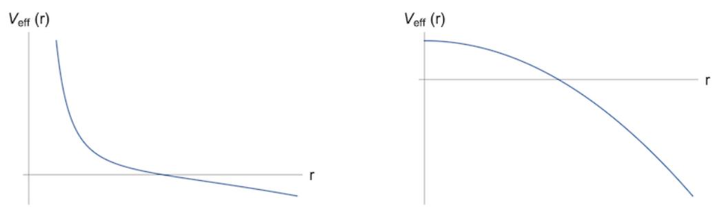
Figure 20. The effective potential for a massive particle in de Sitter with angular momentum (on the left) and with no angular momentum (on the right).

where the effective potential is given by

$$V_{\mathrm{eff}}(r)=\left(1+\frac{l^2}{r^2}\right)f(r{)}^2$$

For geodesics in de Sitter, we therefore have

$$V_{\mathrm{eff}}(r)=\left(1+\frac{l^2}{r^2}\right)\left(1-\frac{r^2}{R^2}\right)$$

This is shown in the figures for $l\ne 0$ and for $l=0$ . We can immediately see the key physics: the potential pushes the particle out to larger values of $r.$ .

We focus on geodesics with vanishing angular momentum, $l=0$ . In this case, the potential is an inverted harmonic oscillator. A particle sitting stationary at $r=0$ is a geodesic, but it is unstable: if it has some initial velocity then it will move away from the origin, following the trajectory

$$r(\sigma )=R\sqrt{E^2-1}\sinh \left(\frac{\sigma }{R}\right)\text{\hspace{1em}(4.15)}$$

The metric (4.12) is singular at $r=R,$ which might make us suspect that something fishy is going on there. But whatever this fishiness is, it’s not visible in the solution (4.15) which shows that any observer reaches $r=R$ in finite proper time $\sigma .$

The fishiness reveals itself if we look at the coordinate time t. This also has the interpretation of the time experienced by someone sitting at the point $r=0$ . Using (4.14), the trajectory (4.15) evolves as

$$\frac{dt}{d\sigma }=E{\left(1-\frac{r^2}{R^2}\right)}^{-1}$$

It is simple to check that $t(\sigma )\to \infty$ as $r(\sigma )\to R$ . (For example, suppose that we have $r(\sigma )=R$ at some value $\sigma ={\sigma }_{\star }$ of proper time. Then look at what happens just before this time by expanding $\sigma ={\sigma }_{\star }-ϵ$ with ϵ small. The equation above becomes $dt/dϵ=-\alpha /ϵ$ for some constant $\alpha ,$ , telling us that $t(ϵ)\sim -\log (ϵ/R)$ and we indeed find that $t\to \infty \mathrm{as}ϵ\to 0.)$ This means that while a guy on the trajectory (4.15) sails right through the point $r=R$ in finite proper time, according to his companion waiting at $r=0$ this will take infinite time.

This strange behaviour is, it turns out, similar to what happens at the horizon of a black hole, which is the surface $r=2GM$ in the metric (4.8). (We will look at more closely at this in Section 6.) However, the Schwarzschild metic also has a singularity at $r=0$ , whereas the de Sitter metric looks just like flat space at $r=0$ . (To see this, simply Taylor expand the coefficients of the metric around $r=0.)$ Instead, de Sitter space seems like an inverted black hole in which particles are pushed outwards to $r=R$ . But how should we interpret this radius? We will get more intuition for this as we proceed.

de Sitter Embeddings

We will have to wait until Section 4.4.2 to get a full understanding of the physics behind this. But we can make some progress by writing the de Sitter metric in different coordinates. In fact, it turns out that there’s a rather nice way of embedding de Sitter space as a sub-manifold of ${\mathbf{R}}^{1,4}$ , with metric

$$d{s}^2=-(d{X}^0{)}^2+\sum _{i=1}^4(d{X}^i{)}^2\text{\hspace{1em}(4.16)}$$

We will now show that the de Sitter space metric (4.12) is a metric on the sub-manifold in ${\mathbf{R}}^{1,4}$ defined by the timelike hyperboloid

$$-(X^0{)}^2+\sum _{i=1}^4(X^i{)}^2=R^2\text{\hspace{1em}(4.17)}$$

There are a number of different ways to parameterise solutions to this constraint. Suppose that we choose to treat $X^4$ as a special coordinate. We define the sum of the first three spatial coordinates to be

$$r^2=(X^1{)}^2+(X^2{)}^2+(X^3{)}^2\text{\hspace{1em}(4.18)}$$

so the constraint (4.17) becomes

$$R^2-r^2=-(X^0{)}^2+(X^4{)}^2$$

We can parameterise solutions to this equation as

$$X^0=\sqrt{R^2-r^2}\sinh (t/R)\mathrm{and}{X}^4=\sqrt{R^2-r^2}\cosh (t/R)\text{\hspace{1em}(4.19)}$$

The variation is then

$$\begin{array}{rl}& d{X}^0=\sqrt{1-\frac{r^2}{R^2}}\cosh (t/R)dt-\frac{r}{\sqrt{R^2-r^2}}\sinh (t/R)dr\\ & d{X}^4=\sqrt{1-\frac{r^2}{R^2}}\sinh (t/R)dt-\frac{r}{\sqrt{R^2-r^2}}\cosh (t/R)dr\end{array}$$

Meanwhile the variation of $X^i$ , with $i=1,2,3,$ is just the familiar line element for ${\mathbf{R}}^3$ : ${\sum }_{i=1}^3(d{X}^i{)}^2=d{r}^2+r^{2}d{\Omega }_2^2$ where $d{\Omega }_2^2$ is the metric on the unit 2-sphere. A two line calculation then shows that the pull-back of the 5d Minkowski metric (4.16) onto the hypersurface (4.17) gives the de Sitter metric in the static patch coordinates (4.12).

The choice of coordinates (4.18) and (4.19) are not the most intuitive. First, they single out $X^4$ as special, when the constraint (4.17) does no such thing. This hides some of the symmetry of de Sitter space. Moreover, the coordinates do not cover the whole of the hyperboloid, since they restrict only to $X^4\ge 0$

We can do better. Consider instead the solution to the constraint (4.17)

$$X^0=R\sinh (\tau /R)\text{ and }{X}^i=R\cosh (\tau /R)y^i\text{\hspace{1em}(4.20)}$$

where the $y^i$ , with $i=1,2,3,4.$ , obey $\begin{array}{r}{\sum }_i(y^i{)}^2=1\end{array}$ and so parameterise a unit 3-sphere. These coordinates have the advantage that they retain (more of) the symmetry of de Sitter space, and cover the whole space. Substituting this into the 5d Minkowski metric (4.16) gives a rather different metric on de Sitter space,

$$d{s}^2=-d{\tau }^2+R^2{\cosh }^2(\tau /R)d{\Omega }_3^2\text{\hspace{1em}(4.21)}$$

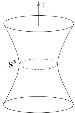
where $d{\Omega }_3^2$ denotes the metric on the unit 3-sphere. These are known as global coordinates, since they cover the whole space. (Admittedly, any choice of coordinates on ${\mathbf{S}}^3$ will suffer from the familiar problem of coordinate singularities at the poles.) Since this metric is related to (4.12) by a change of coordinates, it too must obey the Einstein equation. (We’ll check this explicitly in Section 4.6 where we discuss a class of metrics of this form.)

These coordinates provide a much clearer intuition for the physics of de Sitter space: it is a time-dependent solution in which a spatial ${\mathbf{S}}^3$ first shrinks to a minimal radius $R,$ and subsequently expands. This is shown in the figure. The expansionary phase is a fairly good approximation to our current universe on large scales; you can learn more about this in the lectures on Cosmology.

The cosmological interpretation of an expanding universe is much harder to glean from the static patch coordinates (4.12) in which the space appears to be unchanging in time. Indeed, de Sitter himself originally discovered the metric in the static patch coordinates. He noticed that light is redshifted in this metric, which then caused all sorts of confusion when trying to understand whether the redshift of galaxies (then known as the de Sitter effect!) should be viewed as evidence for an expanding universe. There is a lesson here: it can

be difficult to stare at a metric and get a sense for what you’re looking at.

The global coordinates clearly show that there is nothing fishy happening when $X^4=0$ , the surface which corresponds to $r=R$ in (4.12). This is telling us that this is nothing but a coordinate singularity. (As, indeed, is the $r=2GM$ singularity in the Schwarzschild metric.) Nonetheless, there is still some physics lurking in this coordinate singularity, which we will extract over the next few sections.

4.2.2 Anti-de Sitter Space

We again look for solutions to the Einstein equations,

$$R_{\mu \nu }=\Lambda g_{\mu \nu }$$

now with a negative cosmological constant $\Lambda <0$ . We can again use the ansatz (4.9) and again find the constraints (4.10) and (4.11). The fact that Λ is now negative means that our previous version of $f(r)$ no longer works, but it’s not hard to find the tweak: the resulting metric takes the form

$$d{s}^2=-\left(1+\frac{r^2}{R^2}\right)d{t}^2+{\left(1+\frac{r^2}{R^2}\right)}^{-1}d{r}^2+r^2(d{\theta }^2+{\sin }^2\theta d{\varphi }^2)\text{\hspace{1em}(4.22)}$$

with $R^2=-3/\Lambda$ . This is the metric of anti-de Sitter space, also known simply as AdS.

Sometimes this metric is written by introducing the coordinate $r=R$ sinh $\rho ,$ after which it takes the form

$$d{s}^2=-{\cosh }^2\rho d{t}^2+R^{2}d{\rho }^2+R^2{\sinh }^2\rho (d{\theta }^2+{\sin }^2\theta d{\varphi }^2)\text{\hspace{1em}(4.23)}$$

Now there’s no mysterious coordinate singularity in the r direction and, indeed, we will see shortly that these coordinates now cover the entire space.

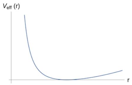
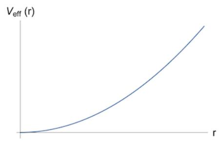
Figure 21. The effective potential for a massive particle in anti-de Sitter with angular momentum (on the left) and with no angular momentum (on the right).

Geodesics in Anti-de Sitter

Because the anti-de Sitter metric (4.22) falls in the general class (4.9), we can import the geodesic equations that we derived for de Sitter space. The radial trajectory of a massive particle moving in the $\theta =\pi /2$ plane is again governed by

$${\dot{r}}^2+V_{\mathrm{eff}}(r)=E^2\text{\hspace{1em}(4.24)}$$

but this time with the effective potential

$$V_{\mathrm{eff}}(r)=\left(1+\frac{l^2}{r^2}\right)\left(1+\frac{r^2}{R^2}\right)$$

Again, $l=r^2\dot{\varphi }$ is the angular momentum of the particle. This potential is shown in the figures for $l\ne 0$ and $l=0$ . From this, we can immediately see how geodesics behave. If there is no angular momentum, so $l=0$ , anti-de Sitter space acts like a harmonic potential, pushing the particle towards the origin $r=0$ . Geodesics oscillate backwards and forwards around $r=0$

In contrast, if the particle also has angular momentum then the potential has a minimum at $r_{\star }^2=Rl$ . This geodesic is like a motorcycle wall-of-death trick, with the angular momentum keeping the particle pinned up the potential. Other geodsics spin in the same fashion, while oscillating about $r_{\star }$ . Importantly, particles with finite energy E cannot escape to $r\to \infty ;$ they are trapped by the spacetime to live within some finite distance of the origin.

The picture that emerges from this analysis is that AdS is like a harmonic trap, pushing particles to the origin. This comes with something of a puzzle however because, as we will see below (and more in Section 4.3), AdS is a homogeneous space which, roughly speaking, means that all points are the same. How is it possible that AdS acts like a harmonic trap, pushing particles to $r=0$ , yet is also a homogeneous space?!

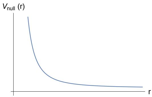
Figure 22. The potential experienced by massless particles in AdS.

To answer this question, consider a guy sitting stationary at the origin $r=0$ . This is a geodesic. From his perspective, intrepid AdS explorers on other geodesics (with, say, $l=0)$ will oscillate backwards and forwards about the origin $r=0$ , just like a particle in a harmonic trap. However, since these explorers will themselves be travelling on a geodesic, they are perfectly entitled to view themselves as sedentary, stay-at-home types, sitting perfectly still at their ‘origin’, watching the other folk fly around them. In this way, just as everyone in de Sitter can view themselves at the centre of the universe, with other observers moving away from them, everyone in anti-de Sitter can view themselves in the centre of the universe, with other observers flying around them.

We can also look at the fate of massless particles. This time the action is supplemented by the constrain

$$-f(r{)}^2{\dot{t}}^2+f(r{)}^{-2}{\dot{r}}^2+r^2({\dot{\theta }}^2+{\sin }^2\theta {\dot{\varphi }}^2)=0$$

This tells us that the particle follows a null geodesic. The equation (4.24) gets replaced by

$${\dot{r}}^2+V_{\mathrm{null}}(r)=E^2$$

with the effective potential now given by

$$V_{\mathrm{null}}(r)=\frac{l^2}{r^2}\left(1+\frac{r^2}{R^2}\right)$$

This potential is again shown in Figure 22. This time the potential is finite as $r\to \infty$ 2 which tells us that there is no obstacle to light travelling as far as it likes: it suffers only the usual gravitational redshift. We learn that AdS spacetime confines massive particles, but not massless ones.

To solve the equations for a massless particle, it’s simplest to work in the coordinates $r=R\sinh \rho$ that we introduced in (4.23). If we restrict to vanishing angular momentum, $l=0$ , the equation above becomes

$$R\dot{\rho }=\pm \frac{E}{\cosh \rho }\Rightarrow R\sinh \rho =E(\sigma -{\sigma }_0)$$

where $\sigma$ is the affine geodesic parameter. We see that $\rho \to \infty$ only in infinite affine time, $\sigma \to \infty$ . However, it’s more interesting to see what happens in coordinate time. This follows by recalling the definition of E in (4.14),

$$E={\cosh }^2\rho \dot{t}$$

(Equivalently, you can see this by dint of the fact that we have a null geodesic, with coshρ $\dot{t}=\pm R\dot{\rho }.)$ We then find

$$R\tan (t/R)=E(\sigma -{\sigma }_0)$$

So as $\sigma \to \infty$ , the coordinate time tends to $t\to \pi R/2$ . We learn that not only do light rays escape to $\rho =\infty$ , but they do so in a finite coordinate time t. This means that to make sense of dynamics in AdS, we must specify some boundary conditions at infinity to dictate what happens to massless particles or fields when they reach it.

Anti-de Sitter space does not appear to have any cosmological applications. However, it turns out to be the place where we best understand quantum gravity, and so has been the object of a great deal of study.

Anti-de Sitter Embeddings

Like its $\Lambda >0$ cousin, anti-de Sitter spacetime also has a natural embedding in a 5d spacetime. This time, it sits within ${\mathbf{R}}^{2,3}$ , with metric

$$d{s}^2=-(d{X}^0{)}^2-(d{X}^4{)}^2+\sum _{i=1}^3(d{X}^i{)}^2\text{\hspace{1em}(4.25)}$$

where it lives as the hyperboloid,

$$-(X^0{)}^2-(X^4{)}^2+\sum _{i=1}^3(X^i{)}^2=-R^2\text{\hspace{1em}(4.26)}$$

We can solve this constraint by

$$X^0=R\cosh \rho \sin (t/R),X^4=R\cosh \rho \cos (t/R),X^i=R{y}^i\sinh \rho \text{\hspace{1em}(4.27)}$$

where the $y^i$ , with $i=1,2,3$ , obey $\begin{array}{r}{\sum }_i(y^i{)}^2=1\end{array}$ and so parameterise a unit 2-sphere. Substituting this into the metric (4.25) gives the anti-de Sitter metric in the coordinates (4.23).

In fact there is one small subtlety: the embedding hyperboloid has topology ${\mathbf{S}}^1\times$ ${\mathbf{R}}^3$ , with ${\mathbf{S}}^1$ corresponding to a compact time direction. This can be seen in the parameterisation (4.27), where the time coordinate takes values $t\in [0,2\pi R)$ . However, the AdS metrics (4.22) or (4.23) have no such restriction, with $t\in (-\infty ,+\infty )$ . They are the universal covering of the hyperboloid (4.26).

There is another parameterisation of the hyperboloid that is also useful. It takes the rather convoluted form

$$X^i=\frac{r}{R}{x}^i\mathrm{for}i=0,1,2,X^4-X^3=r,X^4+X^3=\frac{R^2}{r}+\frac{r}{R^2}{\eta }_{ij}{x}^i{x}^j$$

with $r\in [0,\infty )$ . Although the change of coordinates is tricky, the metric is very straightforward, taking the form

$$d{s}^2=R^2\frac{d{r}^2}{r^2}+\frac{r^2}{R^2}{\eta }_{ij}d{x}^{i}d{x}^j\text{\hspace{1em}(4.28)}$$

These coordinates don’t cover the whole of AdS; instead they cover only one-half of the hyperboloid, restricted to $X^4-X^3>0$ . This is known as the Poincar´e patch of AdS. Moreover, the time coordinate, which already extends over the full range $x^0\in$ $(-\infty ,+\infty )$ , cannot be further extended. This means that as $x^0$ goes from −∞ to +∞ in (4.28), in global coordinates (4.22), the time coordinate t goes only from 0 to $2\pi R$

Two other choices of coordinates are also commonly used to describe the Poincar´e patch. If we set $z=R^2/r$ , then we have

$$d{s}^2=\frac{R^2}{z^2}\left(d{z}^2+{\eta }_{ij}d{x}^{i}d{x}^j\right)$$

Alternatively, if we set $r=R{e}^{\rho }$ , we have

$$d{s}^2=R^{2}d{\rho }^2+e^{2\rho }{\eta }_{ij}d{x}^{i}d{x}^j$$

In each case, massive particles fall towards $r=0$ , or $z=\infty$ , or $\rho =-\infty$

来源与版本

正文：英文 · OCR 机器稿 · 待校对

核对状态：OCR 机器稿 · 待校对

原书 PDF

来源版本：michaelmas-2019-source-20260923

来源 PDF SHA-256：3ba65dc61f22a69c7d5fdf3e8e1f641efbfa6cf49a44b3dcb0fd5367ba9fcf1c

OCR 来源 SHA-256：988fe63d50521107cf7e476ccf517496c8ba2ca839cea1e6e9e5e0bcf9ce0f79

OCR 产物 SHA-256：4822c4221fbfe0caf3db982a62caee9b412cc700ca839d3c5a240967e11953e1