4.4 Asymptotics of Spacetime

The three solutions – Minkowski, de Sitter, and anti-de Sitter – have different spacetime curvature and differ in their symmetries. But there is a more fundamental distinction: they have different behaviour at infinity.

This is important because we will ultimately want to look at more complicated solutions. These may have reduced symmetries, or no symmetries at all. But, providing fields are suitably localised, they will asymptote to one of the three symmetric spaces described above. This gives us a way to characterise whether physics is happening “in Minkowski spacetime”, “in de Sitter”, or “in anti-de Sitter”.

It turns out that “infinity” in Lorentzian spacetimes is more interesting than you might have thought. One can go to infinity along spatial, timelike or null directions, and each of these may have a different structure. It will be useful to introduce a tool to visualise infinity of spacetime.

4.4.1 Conformal Transformations

Given a spacetime M with metric $g_{\mu \nu }$ , we may construct a new metric ${\tilde{g}}_{\mu \nu }$ by a conformal transformation,

$${\tilde{g}}_{\mu \nu }(x)={\Omega }^2(x)g_{\mu \nu }(x)\text{\hspace{1em}(4.34)}$$

with $\Omega (x)$ a smooth, non-vanishing function.

Typically $g_{\mu \nu }$ and ${\tilde{g}}_{\mu \nu }$ describe very different spacetimes, with distances in the two considerably warped. However, the conformal transformation preserves angles. In particular, in a Lorentzian spacetime, this means that two metrics related by a conformal transformation have the same causal structure. A vector field X which is everywherenull with respect to the metric $g_{\mu \nu }$ will also be everywhere-null with respect to ${\tilde{g}}_{\mu \nu }$ ，

$$g_{\mu \nu }{X}^{\mu }{X}^{\nu }=0\iff {\tilde{g}}_{\mu \nu }{X}^{\mu }{X}^{\nu }=0$$

Similarly, vectors that are timelike/spacelike with respect to $g_{\mu \nu }$ will continue to be timelike/spacelike separated with respect to ${\tilde{g}}_{\mu \nu }$

A conformal transformation of the metric does not change the causal structure. However, any other change of the metric does. This fact is sometimes summarised in the slogan “the causal structure is $9/10^{\mathrm{th}}$ of the metric”. Although, taking into account diffeomorphism invariance, a better slogan would be “the causal structure is around $5/6^{\mathrm{th}}$ of the metric”.

Conformal Transformations and Geodesics

A particle trajectory which is timelike with respect to $g_{\mu \nu }$ will necessarily also be timelike with respect to ${\tilde{g}}_{\mu \nu }$ . But because distances get screwed up under a conformal transformation, there is no reason to expect that a timelike geodesic will map to a timelike geodesic. However, it turns out that null geodesics do map to null geodesics, although the affine parameterisation gets messed up along the way.

To see this, we first compute the Christoffel symbols in the new metric. They are

$$\begin{array}{rl}& {\Gamma }_{\rho \sigma }^{\mu }[\tilde{g}]=\frac{1}{2}{\tilde{g}}^{\mu \nu }({\partial }_{\rho }{\tilde{g}}_{\nu \sigma }+{\partial }_{\sigma }{\tilde{g}}_{\rho \nu }-{\partial }_{\nu }{\tilde{g}}_{\rho \sigma })\\ & =\frac{1}{2}{\Omega }^{-2}{g}^{\mu \nu }({\partial }_{\rho }({\Omega }^2{g}_{\nu \sigma })+{\partial }_{\sigma }({\Omega }^2{g}_{\rho \nu })-{\partial }_{\nu }({\Omega }^2{g}_{\rho \sigma }))\\ & ={\Gamma }_{\rho \sigma }^{\mu }[g]+{\Omega }^{-1}({\delta }_{\sigma }^{\mu }{\nabla }_{\rho }\Omega +{\delta }_{\rho }^{\mu }{\nabla }_{\sigma }\Omega -g_{\rho \sigma }{\nabla }^{\mu }\Omega )\end{array}$$

where, in the final line, we’ve replaced ∂ with $\nabla$ on the grounds that the derivatives are hitting a scalar function $\Omega (x)$ so it makes no difference.

If we have an affinely parameterised geodesic in the metric $g$

$$\frac{d^2{x}^{\mu }}{d{\tau }^2}+{\Gamma }_{\rho \sigma }^{\mu }[g]\frac{d{x}^{\rho }}{d\tau }\frac{d{x}^{\sigma }}{d\tau }=0$$

then in the metric $\tilde{g}$ we have

$$\frac{d^2{x}^{\mu }}{d{\tau }^2}+{\Gamma }_{\rho \sigma }^{\mu }[\tilde{g}]\frac{d{x}^{\rho }}{d\tau }\frac{d{x}^{\sigma }}{d\tau }={\Omega }^{-1}\left({\delta }_{\sigma }^{\mu }{\nabla }_{\rho }\Omega +{\delta }_{\rho }^{\mu }{\nabla }_{\sigma }\Omega -g_{\rho \sigma }{\nabla }^{\nu }\Omega \right)\frac{d{x}^{\rho }}{d\tau }\frac{d{x}^{\sigma }}{d\tau }$$

The right-hand side looks like a mess. And for timelike or spacelike geodesics, it is. But for null geodesics we have

$$g_{\rho \sigma }\frac{d{x}^{\rho }}{d\tau }\frac{d{x}^{\sigma }}{d\tau }=0$$

so at least one term on the right-hand side vanishes. The others can be written as

$$\frac{d^2{x}^{\mu }}{d{\tau }^2}+{\Gamma }_{\rho \sigma }^{\mu }[\tilde{g}]\frac{d{x}^{\rho }}{d\tau }\frac{d{x}^{\sigma }}{d\tau }=2\frac{d{x}^{\mu }}{d\tau }\frac{1}{\Omega }\frac{d\Omega }{d\tau }$$

But this is the equation for a geodesic that is not affinely parameterised, as in (1.28). So a conformal transformation does map null geodesics to null geodesics as claimed.

The Weyl Tensor

Our favourite curvature tensors are not invariant under conformal transformations. However, it turns out that there is a combination of curvature tensors that does not change under conformal transformations. This is the Weyl tensor. In a manifold of dimension n, it is defined as

$$C_{\mu \nu \rho \sigma }=R_{\mu \nu \rho \sigma }-\frac{2}{n-2}\left(g_{\mu [\rho }{R}_{\sigma ]\nu }-g_{\nu [\rho }{R}_{\sigma ]\mu }\right)+\frac{2}{(n-1)(n-2)}R{g}_{\mu [\rho }{g}_{\sigma ]\nu }$$

The Weyl tensor has all the symmetry properties of the Riemann tensor, but with the additional property that if you contract any pair of indices with a metric then it vanishes. In this sense, it can be viewed as the “trace-free” part of the Riemann tensor.

4.4.2 Penrose Diagrams

There are a number of interesting and deep stories associated to conformal transformations (4.34). For example, there are a class of theories that are invariant under conformal transformations of Minkowski space; these so-called conformal field theories describe physics at a second order phase transition. But here we want to use conformal transformations to understand what happens at infinity of spacetime.

The main idea is to perform a conformal transformation that pulls infinity to some more manageable, finite distance. Obviously this transformation will mangle distances, but it will retain the causal structure of the original spacetime. We can then draw this causal structure on a very finite piece of paper (e.g. A4). The resulting picture is called a Penrose diagram, named after its discoverers, Roger Penrose and Brandon Carter. We will illustrate this with a series of examples.

Minkowski Space

We start with Minkowski space. It turns out that, even here, infinity is rather subtle.

It will be simplest if we first work in $d=1+1$ dimensions, where the Minkowski metric takes the form

$$d{s}^2=-d{t}^2+d{x}^2\text{\hspace{1em}(4.35)}$$

The first thing we do is introduce light-cone coordinates,

$$u=t-x\mathrm{and}v=t+x$$

In these coordinates, the Minkowski metric is even simpler

$$d{s}^2=-dudv$$

Both of these light-cone coordinates take values over the full range of R: $u,v\in$ $(-\infty ,\infty )$ . In an attempt to make things more finite, we will introduce another coordinate that traverses the full range of $u$ and $v$ over a finite interval. A convenient choice is

$$u=\tan \tilde{u}\mathrm{and}v=\tan \tilde{v}\text{\hspace{1em}(4.36)}$$

where we now cover the whole of Minkowski space as ˜u, $\tilde{v}\in (-\pi /2,+\pi /2)$ . Note that, strictly speaking, we shouldn’t include the points $\tilde{u},\tilde{v}=\pm \pi /2$ since these correspond to $u,v=\pm \infty$

In the new coordinates, the metric takes the form

$$d{s}^2=-\frac{1}{{\cos }^2\tilde{u}{\cos }^2\tilde{v}}d\tilde{u}d\tilde{v}$$

Notice that the metric diverges as we approach the boundary of Minkowski space, where $\tilde{u}$ or $\tilde{v}\to \pm \pi /2$ . However, we can now do our conformal transformation. We define the new metric

$$d{\tilde{s}}^2=({\cos }^2\tilde{u}{\cos }^2\tilde{v})d{s}^2=-d\tilde{u}d\tilde{v}$$

After the conformal map, nothing bad happens as we approach $\tilde{u},\tilde{v}\to \pm \pi /2$ . It is customary to now add in the “points at infini $;{\mathrm{y}}^{†}$ , $\tilde{u}=\pm \pi /2$ and $\tilde{v}=\pm \pi /2$ , an operation that goes by the name of conformal compactification.

The Penrose diagram is a pictorial representation of this space. As in other relativistic diagrams, we insist that light-rays go at $45^{\circ }$ . We take time to be in the vertical direction, and space in the horizontal. This means that we draw the lightcone $\tilde{u}$ and $\tilde{v}$ coordinates at $45^{\circ }$ . The resulting diagram is shown with the $\tilde{u}$ and $\tilde{v}$ axes on the left-hand side of Figure 23.

We can also dress our Penrose diagram in various ways. For example, we could draw geodesics with respect to the original metric (4.35). These are shown in the right-hand side of Figure 23; the verticalish blue lines are timelike geodesics of constant $x;$ the horizontalish red lines are spacelike geodesics of constant t. We have also listed the different kinds of “infinity” for Minkowski space. They are

• All timelike geodesics start at the point labelled $i^{-}$ , with $(\tilde{u},\tilde{v})=(-\pi /2,-\pi /2)$ and end at the point labelled $i^{+}$ with $(\tilde{u},\tilde{v})=(+\pi /2,+\pi /2)$ . In other words, this is the origin and fate of all massive particles. These points are referred to as past and future timelike infinity respectively.

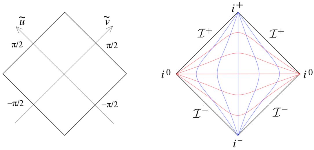
Figure 23. The Penrose diagram for $d=1+1$ Minkowski space.

• All spacelike geodesics begin or end at one of the two points labelled $i^0$ , either $(\tilde{u},\tilde{v})=(-\pi /2,+\pi /2)$ or $(\tilde{u},\tilde{v})=(+\pi /2,-\pi /2)$ . These points are spacelike infinity.

• All null curves start on the boundary labelled ${\mathcal{I}}^{-}$ , with $\tilde{u}=-\pi /2$ and arbitrary $\tilde{v}$, or $\tilde{v}=-\pi /2$ and arbitrary $\tilde{u}.$ . This boundary is pronounced “scri-minus” and known, more formally, as past null infinity. Such null curves end on the boundary labelled ${\mathcal{I}}^{+}$ , with $\tilde{u}=+\pi /2$ and arbitrary $\tilde{v},$ or $\tilde{v}=+\pi /2$ and arbitrary $\tilde{u}.$ This is pronounced “scri-plus” and known as future null infinity.

We see from the picture that there are more ways to ${}^{66}\mathrm{go}$ to infinity” in a null direction than in a timelike or spacelike direction. This is one of the characteristic features of Minkowski space.

The Penrose diagram allows us to immediately visualise the causal structure of Minkowski space. For example, as timelike curves approach $i^{+}$ , their past lightcone encompasses more and more of the spacetime, as shown in the left-hand side of Figure 24. This means that an observer in Minkowski space can see everything (in principle) as long as they wait long enough. Relatedly, given any two points in Minkowski space, they are causally connected in both the past and future, meaning that their past and future lightcones necessarily intersect, as shown in the Mondrian painting on the righthand side of Figure 24. This means that there was always an event in the past that could influence both points, and always an event in the future that can be influenced by both. These comments may seem trivial, but we will soon see that they don’t hold in other spacetimes, including the one we call home.

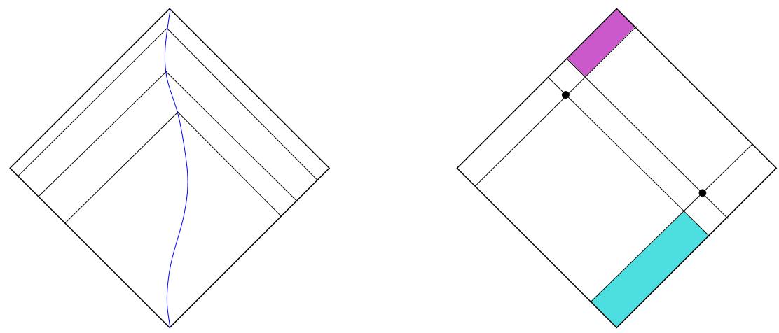
Figure 24. On the left: you will eventually see everything. On the right: every two points share some of their causal past and some of their causal future.

Let’s now repeat the analysis for Minkowski space in $d=3+1$ dimensions, with the metric

$$d{s}^2=-d{t}^2+d{r}^2+r^{2}d{\Omega }_2^2$$

where $d{\Omega }_2^2=d{\theta }^2+{\sin }^2\theta d{\varphi }^2$ is the round metric on ${\mathbf{S}}^2$ (and is not to be confused with the conformal factor $\Omega (x)$ that we introduced earlier). Again we introduce lightcone coordinates

$$u=t-r\mathrm{and}v=t+r$$

and write this metric as

$$d{s}^2=-dudv+\frac{1}{4}(u-v{)}^{2}d{\Omega }_2^2$$

In the finite-range coordinates (4.36), the metric becomes

$$d{s}^2=\frac{1}{4{\cos }^2\tilde{u}{\cos }^2\tilde{v}}\left(-4d\tilde{u}d\tilde{v}+{\sin }^2(\tilde{u}-\tilde{v})d{\Omega }_2^2\right)$$

Finally, we do the conformal transformation to the new metric

$$d{\tilde{s}}^2=-4d\tilde{u}d\tilde{v}+{\sin }^2(\tilde{u}-\tilde{v})d{\Omega }_2^2\text{\hspace{1em}(4.37)}$$

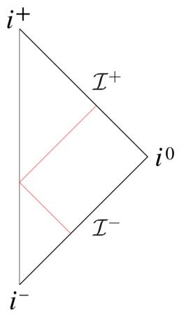
Figure 25. The Penrose diagram for 4d Minkowski spacetime.

There is an additional requirement that didn’t arise in $2\mathrm{d}:$ we must insist that $v\ge u$ so that $r\ge 0$ , as befits a radial coordinate. This means that, after a conformal compactification, ˜u and $\tilde{v}$ take values in

$$-\frac{\pi }{2}\le \tilde{u}\le \tilde{v}\le \frac{\pi }{2}$$

To draw a diagram corresponding to the spacetime (4.37), we’re going to have to ditch some dimensions. We chose not to depict the ${\mathbf{S}}^2$ , and only show the ˜u and ˜v directions. The resulting Penrose diagram for $d=3+1$ dimensional Minkowski space is shown in Figure 25.

Every point in the diagram corresponds to an ${\mathbf{S}}^2$ of radius sin $(\tilde{u}-\tilde{v})$ , except for the left-hand line which sits at $\tilde{u}=\tilde{v}$ where this ${\mathbf{S}}^2$ shrinks to a point. This is not a boundary of Minkowski space; it is simply the origin $r=0$ . To illustrate this, we’ve drawn a null geodesic in red in the figure; it starts at ${\mathcal{I}}^{-}$ and and when it hits the $r=0$ vertical line, it simply bounces of and ends up at ${\mathcal{I}}^{+}$

The need to draw a 4d space on a 2d piece of paper is something of a limitation of Penrose diagrams. It means that they’re only really useful for spacetimes that have an obvious ${\mathbf{S}}^2$ sitting inside them that we can drop. Or, to state it more precisely, spacetimes that have an $SO(3)$ isometry. But these spacetimes are the simplest and tend to be the most important.

We have seen that Minkowski space has a null boundary, together with a couple of points at spatial and temporal infinity. This naturally lends itself to asking questions about scattering of massless fields: we set up some initial data on ${\mathcal{I}}^{-}$ , let it evolve, and read of its fate at ${\mathcal{I}}^{+}$ . In quantum field theory, this is closely related to the object we call the S-matrix.

de Sitter Space

The global coordinates for de Sitter space are (4.21),

$$d{s}^2=-d{\tau }^2+R^2{\cosh }^2(\tau /R)d{\Omega }_3^2$$

To construct the Penrose diagram we work with conformal time, defined by

$$\frac{d\eta }{d\tau }=\frac{1}{R\cosh (\tau /R)}$$

The solution is

$$\cos \eta =\frac{1}{\cosh (\tau /R)}\text{\hspace{1em}(4.38)}$$

with $\eta \in \left(-\pi /2,+\pi /2\right)$ as $\tau \in (-\infty ,+\infty )$ . In conformal time, de Sitter space has the metric

$$d{s}^2=\frac{R^2}{{\cos }^2\eta }\left(-d{\eta }^2+d{\Omega }_3^2\right)$$

We write the metric on the ${\mathbf{S}}^3$ as

$$d{\Omega }_3^2=d{\chi }^2+{\sin }^2\chi d{\Omega }_2^2\text{\hspace{1em}(4.39)}$$

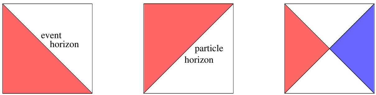
Figure 27. On the left: an observer at the north pole does not see everything. She has an event horizon. In the middle: Nor can she influence everything: she has a particle horizon. On the right: the causal diamond for an observer at the north pole (in red) and at the south pole (in blue).

with $\chi \in [0,\pi ]$ . The de Sitter metric is conformally equivalent to

$$d{\tilde{s}}^2=-d{\eta }^2+d{\chi }^2+{\sin }^2\chi d{\Omega }_2^2$$

After a conformal compactification, $\eta \in \left[-\pi /2,+\pi /2\right]$ and $\chi \in [0,\pi ]$ . The Penrose diagram is shown in Figure 26.

The two vertical lines are not boundaries of the spacetime; they are simply the north and south poles of the ${\mathbf{S}}^3$ . The boundaries are the horizontal lines at the top and bottom: they are labelled both as $i^{\pm }$ and ${\mathcal{I}}^{\pm }$ , reflecting the fact that they are where both timelike and null geodesics originate and terminate.

We learn that de Sitter spacetime has a spacelike ${\mathbf{S}}^3$ boundary. (The normal to this boundary is timelike.)

The causal structure of de Sitter spacetime is very different from Minkowski. It is not true that if an observer waits long enough then she will be able to see everything that’s happening. For example, an observer who sits at the north pole (the left-hand side of the figure) will ultimately be able to see exactly half the spacetime, as shown in the left-hand side of Figure 27. The boundary of this space (the diagonal line in the figure) is her event horizon. It is similar to the event horizon of a black hole in the sense that signals from beyond the horizon cannot reach her. However, as is clear from the picture, it is an observer-dependent horizon: someone else will have an entirely different event horizon. In this context, these are sometimes referred to as cosmological horizons.

Furthermore, the observer at the north pole will only be able to communicate with another half of the spacetime, as shown in the middle of Figure 27. The boundary of the region of influence is known as the particle horizon. You should think of it as the furthest distance light can travel since the beginning of time. The intersection of these two regimes is called the (northern) causal diamond and is shown as the red triangle in the right-hand figure. An observer sitting at the southern pole also has a causal diamond, shown in blue in the right-hand side of Figure 27. It is causally disconnected from the northern diamond.

This state of affairs was nicely summarised by Schr¨odinger who, in 1956, wrote

“It does seem rather odd that two or more observers, even such as sat on the same school bench in the remote past, should in future, when they have followed different paths in life, experience different worlds, so that eventually certain parts of the experienced world of one of them should remain by principle inaccessible to the other and vice versa.”

In asymptotically de Sitter spacetimes, it would appear that the natural questions involve setting some initial conditions on spacelike ${\mathcal{I}}^{-}$ , letting it evolve, and reading of the data on ${\mathcal{I}}^{+}$ . One of the lessons of the development of quantum mechanics is that we shouldn’t talk about things that cannot, even in principle, be measured. Yet in de Sitter space we see that no single observer has an overview of the whole space. This causes a number of headaches and, as yet, unresolved conceptual issues when we try to discuss quantum gravity in de Sitter space.

Finally, we can use the Penrose diagram to answer a lingering puzzle about the static patch of de Sitter, in which the metric takes the form (4.12)

$$d{s}^2=-\left(1-\frac{r^2}{R^2}\right)d{t}^2+{\left(1-\frac{r^2}{R^2}\right)}^{-1}d{r}^2+r^2(d{\theta }^2+{\sin }^2\theta d{\varphi }^2)\text{\hspace{1em}(4.40)}$$

The question is: how should we interpret the divergence at $r=R?$

To answer this, we will look at where the surface $r=R$ sits in the Penrose diagram. First, we look at the embedding of the static patch in ${\mathbf{R}}^{1,4}$ , given in (4.19)

$$X^0=\sqrt{R^2-r^2}\sinh (t/R)\mathrm{and}{X}^4=\sqrt{R^2-r^2}\cosh (t/R)$$

Naively the surface $r=R$ corresponds to $X^0=X^4=0$ . But that’s a little too quick. To see this, we consider what happens as we approach $r\to R$ by writing $r=R(1-{ϵ}^2/2)$ with $ϵ\ll 1$ . We then have

$$X^0\approx Rϵ\sinh (t/R)\text{ and }{X}^4\approx Rϵ\cosh (t/R)$$

We can now send $ϵ\to 0$ , keeping $X^0$ and $X^4$ finite provided that we also send $t\to \pm \infty$ To do this, we must ensure that we keep the combination $ϵe^{\pm t/R}$ finite. This means that we can identify the surface $r=R$ with the lines $X^0=\pm X^4$

Now we translate this into global coordinates. These were given in (4.20),

$$X^0=R\sinh (\tau /R)\mathrm{and}{X}^4=R\cosh (\tau /R)\cos \chi$$

where $\chi$ is the polar angle on ${\mathbf{S}}^3$ that we introduced in (4.39). After one further map to conformal time (4.38), we find that the lines $X^0=\pm X^4$ become

$$\sin \eta =\pm \cos \chi \Rightarrow \chi =\pm (\eta -\pi /2)$$

But these are precisely the diagonal lines in the Penrose diagram that appear as horizons for people living on the poles.

It’s also simple to check that the point $r=0$ in the static patch corresponds to the north pole $\chi =0$ in global coordinates and, furthermore, $t=\tau$ along this line.

The upshot is that the static patch of de Sitter (4.40) provides coordinates that cover only the northern causal diamond of de Sitter, with the coordinate singularity at $r=R$ coinciding with the past and future observer-dependent horizons.

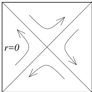
One advantage of the static patch coordinates is that they clearly exhibit a timelike Killing vector, $K={\partial }_t$ . This moves us from a surface of constant t to another surface of constant t. But we argued in Section 4.3.1 that there was no global timelike Killing vector field in de Sitter since, in ${\mathbf{R}}^{1,4}$ , the Killing vector is given by (4.31). The Penrose diagram makes this simpler to visualise. If we extend the Killing vector beyond the static patch, it acts as shown in the figure. It is timelike and future pointing only in the northern causal diamond. It is also timelike in the southern causal diamond, but points towards the past. Meanwhile it is a spacelike Killing vector in both the upper and lower quadrants.

Anti-de Sitter Space

The global coordinates for anti-de Sitter space are (4.23),

$$d{s}^2=-{\cosh }^2\rho d{t}^2+R^{2}d{\rho }^2+R^2{\sinh }^2\rho d{\Omega }_2^2$$

with $\rho \in [0,+\infty )$ . To construct the Penrose diagram, this time we introduce a ${}^{66}\mathrm{con}-$ formal radial coordinate” ψ, defined by

$$\frac{d\psi }{d\rho }=\frac{1}{\cosh \rho }$$

This is very similar to the conformal map of de Sitter space, but with time replaced by space. The solution is

$$\cos \psi =\frac{1}{\cosh \rho }$$

One difference from the de Sitter analysis is that since $\rho \in [0,\infty )$ , the conformal coordinate lives in $\psi \in [0,\pi /2)$ . The metric on anti-de Sitter becomes

$$d{s}^2=\frac{R^2}{{\cos }^2\psi }\left(-d{\tilde{t}}^2+d{\psi }^2+{\sin }^2\psi d{\Omega }_2^2\right)=\frac{R^2}{{\cos }^2\psi }\left(-d{\tilde{t}}^2+d{\Omega }_3^2\right)\text{\hspace{1em}(4.41)}$$

where we’ve introduced the dimensionless time coordinates $\tilde{t}=t/R$ . We learn that the anti-de Sitter metric is conformally equivalent to

$$d{\tilde{s}}^2=-d{\tilde{t}}^2+d{\psi }^2+{\sin }^2\psi d{\Omega }_2^2$$

where, after a conformal compactification, $\tilde{t}\in \mathsf{\Gamma }(-\infty ,+\infty )$ and $\psi \in [0,\pi /2]$ . The resulting Penrose diagram is shown in the left-hand of Figure 28. It is an infinite strip. The left-hand edge at $\psi =0$ is not a boundary: it is the spatial origin where the ${\mathbf{S}}^2$ shrinks to zero size. In contrast, the right-hand edge at $\psi =\pi /2$ is the boundary of spacetime.

The boundary is labelled I. In terms of our previous notation, it should be viewed as a combination of ${\mathbb{T}}^{-},{\mathbb{Z}}^{+}$ and $i^0$ , since null paths begin and end here, as do spacelike paths. The boundary is now timelike (it has spacelike normal vector), and has topology

$$\mathcal{I}=\mathbf{R}\times {\mathbf{S}}^2$$

with R the time factor.

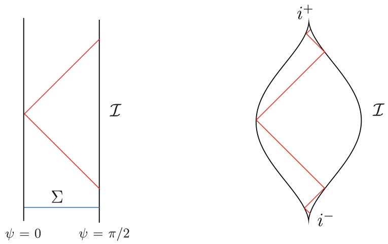
Figure 28. Penrose diagrams for AdS. On the left, we still have an infinite time coordinate; on the right this too has been conformally compactified.

The Penrose diagram allows us to immediately see that light rays hit the boundary in finite conformal time, confirming the calculation that we did in Section 4.2.2. If we want to specify physics in AdS, we need to say something about what happens at the boundary. For example, in the figure we have shown a light ray simply emerging from the boundary at one time and absorbed at some later time. Another choice would be to impose reflecting boundary conditions, so that the light ray bounces back and forth for ever. In this way, anti-de Sitter space is very much like a box, with massive particles trapped in the interior and massless particles able to bounce of the boundary.

In field theoretic language, we could start with initial data on some d = 3 dimensional spacelike hypersurface Σ and try to evolve it in time. This is what we usually do in physics. But in AdS, this information is not sufficient. This is because we can find points to the future of Σ which are in causal contact with the boundary. This means that what happens there depends on the choices we make on the boundary. It’s not particularly difficult to specify what happens on the boundary: for example, we could impose a version of reflecting boundary conditions, so that everything bounces back. But this doesn’t change the fact that we have to specify something and, for this reason, the dynamical evolution is not determined by the initial data alone. In fancy language, we say that AdS is not globally hyperbolic: there exists no Cauchy surface on which we can specify initial data .

AdS is the setting for our best-understood theories of quantum gravity. It turns out that gravitational dynamics in asymptotically AdS spacetimes is entirely equivalent to a quantum field theory living on the boundary I. This idea goes by many names, including the AdS/CFT correspondence, gauge-gravity duality, or simply holography.

Unlike our other Penrose diagrams, our diagram for AdS still stretches to infinity. We can do better. We play our usual trick of introducing a coordinate which runs over finite values, now for time

$$\tilde{t}=\tan \tau \Rightarrow d\tilde{t}=\frac{d\tau }{{\cos }^2\tau }$$

The metric (4.41) then becomes

$$d{s}^2=\frac{R^2}{{\cos }^2\psi {\cos }^4\tau }\left(-d{\tau }^2+{\cos }^4\tau d{\Omega }_3^2\right)$$

where $\tau \in (-\pi /2,+\pi /2)$ . Now we see that AdS is conformally equivalent to

$$d{\tilde{s}}^2=-d{\tau }^2+{\cos }^4\tau \left(d{\psi }^2+{\sin }^2\psi d{\Omega }_2^2\right)$$

Ignoring the spatial ${\mathbf{S}}^2$ , we can draw the resulting Penrose diagram as shown in the right-hand side of Figure 28. Now the spatial ${\mathbf{S}}^3$ grows and shrinks with time, giving the strange almond-shape to the Penrose diagram. Again, we see that there is a timelike boundary $\mathcal{I},$ although now we can also show the future and past timelike infinity, $i^{\pm }$ The diagram again makes it clear that a lightray bounces back and forth an infinite number of times in AdS.

来源与版本

正文：英文 · OCR 机器稿 · 待校对

核对状态：OCR 机器稿 · 待校对

原书 PDF

来源版本：michaelmas-2019-source-20260923

来源 PDF SHA-256：3ba65dc61f22a69c7d5fdf3e8e1f641efbfa6cf49a44b3dcb0fd5367ba9fcf1c

OCR 来源 SHA-256：988fe63d50521107cf7e476ccf517496c8ba2ca839cea1e6e9e5e0bcf9ce0f79

OCR 产物 SHA-256：dce61af110cbd14d928cec4b18bb27ea80601690469e7dadf05fc8f534201c7d