6.3 Rotating Black Holes

In this section, we turn to rotating black holes. These are the appropriate solutions to describe all black holes observed in the universe.

6.3.1 The Kerr Solution

Rotating objects have an axis of rotation, and this necessarily breaks the rotational symmetry. This makes the solution for rotating black holes considerably more complicated than the spherically symmetric solutions that we have discussed so far.

The solution is written in so-called Boyer-Lindquist coordinates $(t,r,\theta ,\varphi )$ . It takes the form

$$d{s}^2=-\frac{\Delta }{{\rho }^2}{\left(dt-a{\sin }^2\theta d\varphi \right)}^2+\frac{{\sin }^2\theta }{{\rho }^2}{\left[(r^2+a^2)d\varphi -adt\right]}^2+\frac{{\rho }^2}{\Delta }d{r}^2+{\rho }^{2}d{\theta }^2\text{\hspace{1em}(6.26)}$$

where $\Delta (r)$ and ${\rho }^2(r,\theta )$ are the following functions

$$\Delta =r^2-2GMr+a^2\mathrm{and}{\rho }^2=r^2+a^2{\cos }^2\theta$$

This is the Kerr solution, written down in 1963. It’s also useful to have an expression for the metric from which we can immediately read of the $g_{tt},{\text{ g }}_{t\varphi }$ and $g_{\varphi \varphi }$ metric components,

$$\begin{array}{rl}& d{s}^2=-\left(1-\frac{2GMr}{{\rho }^2}\right)d{t}^2-\frac{4GMar{\sin }^2\theta }{{\rho }^2}dtd\varphi +\frac{{\rho }^2}{\Delta }d{r}^2\\ & +\frac{{\sin }^2\theta }{{\rho }^2}\left[(r^2+a^2{)}^2-\Delta a^2{\sin }^2\theta \right]d{\varphi }^2+{\rho }^{2}d{\theta }^2\end{array}\text{\hspace{1em}(6.27)}$$

After ploughing through some algebra, you can convince yourself that the Kerr solution has the rather non-obvious property

$$g_{t\varphi }^2-g_{tt}{g}_{\varphi \varphi }=\Delta {\sin }^2\theta \text{\hspace{1em}(6.28)}$$

We’ll make use of this below.

The Kerr solution depends on two parameters: M and a. A quick inspection of the metric shows that a has dimension of length. When $a=0$ , the Kerr solution reduces to the Schwarzschild solution.

Far from the black hole, $r\gg GM,a.$ , the metric reduces to flat Minkowski spacetime, with $(t,r,\theta ,\varphi )$ the usual coordinates, with $\theta \in [0,\pi ]$ and $\varphi \in [0,2\pi )$

There are two continuous isometries of the Kerr metric. These are

$$K=\frac{\partial }{\partial t}\mathrm{and}L=\frac{\partial }{\partial \varphi }$$

We can compute Komar integrals for each of these, giving the mass and angular momentum of the black hole respectively. Unsurprisingly, it turns out that the mass is M. The Komar integral of the rotational Killing vector L gives the angular momentum

$$J=aM$$

Flipping the sign of a changes the direction of the spin. In what follows, we take $a>0$ without loss of generality.

The Schwarzschild solution was also invariant under the discrete symmetries $t\to -t$ and $\varphi \to -\varphi$ The Kerr solution is invariant only under the combination $(t,\varphi )\to$ $(-t,-\varphi )$ , as appropriate for a spinning object.

Black Hole Uniqueness

There are a bunch of theorems, each with slightly different assumptions, that collectively can be summarised as: any time-independent, asymptotically flat black hole solution, lies within the Kerr family. In other words, black holes are characterised by only two numbers: mass M and angular momentum J. (If we are in Einstein-Maxwell theory, these theorems are extended to allow for electric and magnetic charges as well; we’ll briefly discuss this in Section 6.3.4.)

These theorems are not as strong as Birkhoff’s theorem. There we needed only to assume spherical symmetry to land on the Schwarzschild solution. This ensured that the Schwarzschild metric describes the spacetime outside a star, even one that is undergoing spherical collapse.

In contrast, the wider set of theorems make explicit use of the event horizon. This means that the Kerr solution does not necessarily describe the spacetime outside a rotating star, although it seems plausible that it is a good approximation far from the surface of the star.

Nonetheless, these theorems tell us that the end point of gravitational collapse is generically the Kerr black hole. This is rather surprising. General relativity is a classical theory that can be derived from an action principle. In fact, it turns out that it is a Hamiltonian theory. Basic properties of Hamiltonian systems — like Liouville’s theorem — say that the end point of generic evolution can’t be a single point in phase space. Instead, that kind of behaviour is what we expect from a non-Hamiltonian systems with friction. In many ways, black holes act like systems with friction. These kinds of issues become even sharper when we bring quantum mechanics into the mix, where they reappear as the information paradox.

6.3.2 The Global Structure

When $\Delta :=:0$ , the $g_{rr}$ component of the metric diverges. Our previous experience with the Schwarzschild and Reissner-Nordstr¨om black holes suggests that these are coordinate singularities, and this turns out to be correct. We write the roots of $\Delta$ as

$$\Delta =(r-r_{+})(r-r_{-})$$

with

$$r_{\pm }=GM\pm \sqrt{G^2{M}^2-a^2}$$

This has the same structure as the Reissner-Nordstr¨om black hole, and we can immediately import some lessons from there. In particular, if the black hole spins too fast, so $a>GM$ , then the Kerr solution exhibits a naked singularity and is disallowed. The fastest spinning black hole has $a=GM$ and, correspondingly, $J=(GM{)}^2$ . This is the extremal Kerr black hole. More generally, the allowed values of spin are $a/GM\le 1$

To show that $r=r_{\pm }$ are coordinate singularities, we can do something akin to the Eddington-Finkelstein trick. This time things are a little trickier. We introduce the Kerr coordinates $(v,r,\theta ,\chi )$ where $v=t+r_{\star }$ and $r_{\star }$ and $\chi$ defined by

$$d{r}_{\star }=\frac{r^2+a^2}{\Delta }dr\mathrm{and}d\chi =d\varphi +\frac{a}{\Delta }dr\text{\hspace{1em}(6.29)}$$

The idea, once again, is that these coordinates are adapted to null, in-falling geodesics. However, now there are no radial geodesics: instead they get twisted round by the rotation of the black hole. These geodesics don’t, therefore, sit at constant $\varphi$ but instead sit at constant $\chi .$ To see this, we exchange t and $\varphi$ in favour of $v$ and $\chi$ in (6.26) to find

$$d{s}^2=-\frac{\Delta }{{\rho }^2}{\left[dv-a{\sin }^2\theta d\chi \right]}^2+\frac{{\sin }^2\theta }{{\rho }^2}{\left[adv-(r^2+a^2)d\chi \right]}^2+(dv-a{\sin }^2\theta d\chi )dr+{\rho }^{2}d{\theta }^2$$

First, note that null geodesics follow $dv=d\chi =d\theta =0$ as promised (since this ensures that $d{s}^2=0.)$ Second, as with Eddington-Finkelstein coordinates, there is no longer a factor of $\Delta$ in the denominator. This ensures that we can now extend the r coordinate down to $r>0$ without hitting any singularity. We learn that $r=r_{\pm }$ in the original Kerr metric (6.26) were indeed coordinate singularities as advertised.

To build up the full causal structure, we need Kruskal-like coordinates, analogous to the $U_{\pm }$ and $V_{\pm }$ coordinates (6.23) that we introduced for the Reissner-Nordstr¨om black hole. The procedure is now the same. The $U_{+}$ and $V_{+}$ coordinates allow us to extend the spacetime past the outer horizon at $r_{+}$ , down to the inner horizon at $r_{-}$ . We then need to switch to the $U_{-}$ and $V_{-}$ coordinates to get down to the singularity. This then repeats itself. The resulting Penrose diagram again repeats ad infinitum, as shown in Figure 44.

The Singularity

There are a number of ways in which the global structure of the Kerr solution differs from Reissner-Nordstr¨om . One is the singularity. The $g_{tt}$ component of the Kerr metric diverges when

$${\rho }^2=0\Rightarrow r=0\text{ and }\theta =\frac{\pi }{2}$$

From our experience with the Schwarzschild and Reissner-Nordstr¨om black holes, we might expect that this is a true curvature singularity. This is confirmed by an analysis of the Kretschmann scalar.

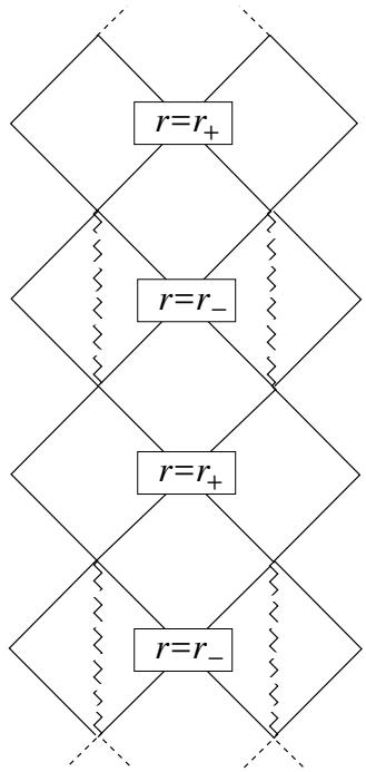
Figure 44. The Penrose diagram for the Kerr black hole.

However, in the previous cases the singularity arose at $r=0$ . There was no need to also specify the angular coordinates on the ${\mathbf{S}}^2$ because the ${\mathbf{S}}^2$ degenerated at $r=0$ just like at the origin of flat space. In contrast, the singularity in Kerr occurs only when $\theta =\pi /2$ . To better understand this, we can look at the Kerr metric (6.26) at $r=0$ , with constant t: it is

$$d{s}^2=a^2{\sin }^2\theta d{\varphi }^2+a^2{\cos }^2\theta d{\theta }^2$$

We see that the ${\mathbf{S}}^2$ has not degenerated at this point, but nor does it have the round metric. This is to be expected, since the Kerr solution did not have rotational symmetry. The restriction to $\theta =\pi /2$ puts us on the “equator”: this is a ring of radius a, parameterised by $\varphi \in [0,2\pi )$ . Thus we learn that the singularity of the Kerr black hole has a ring structure! The singularity is again timelike, as shown in the Penrose diagram.

Strictly speaking, Penrose diagrams can only be drawn for rotationally invariant spacetimes, since we suppress the ${\mathbf{S}}^2$ . For Kerr, we compromise and draw the singularity as the jagged, broken line in Figure 44, reflecting the fact that the singularity only occur when $\theta =\pi /2$ and not for other angles on the ${\mathbf{S}}^2$

Closed Timelike Curves

In the Reissner-Nordstr¨om black hole, the spacetime ended at the timelike singularity. But because the ${\mathbf{S}}^2$ doesn’t degenerate for Kerr, spacetime continues past the singularity (i.e. to the right and left of the timelike singularities shown in Figure 44).

This region can be accessed by observers following a timelike geodesic that passes through $r=0$ at $\theta \ne \pi /2$ . This corresponds to $r<0$ in the original coordinates of (6.26).

This new region has a weird property: it acts as a time machine! To see this, consider a curve which sits at constant t and r and $\theta =\pi /2$ . In other words, the curve is parameterised by $\varphi .$ From (6.26), the metric for this curve is

$$d{s}^2=\left(-\frac{a^2\Delta }{r^2}+\frac{(r^2+a^2{)}^2}{r^2}\right)d{\varphi }^2=\left(r^2+a^2+\frac{2GM{a}^2}{r}\right)d{\varphi }^2$$

For $r<0$ and suitably small, this term in brackets is negative, This means that $\varphi$ is a timelike direction close to the singularity. But $\varphi$ is a periodic coordinate, with $\varphi$ and $\varphi +2\pi$ identified. This means that if you move along this curve, you get back to the same point in time that you started from. This is a closed timelike curve.

Having a time machine tucked away inside a black hole is not going to allow you to play Johnny B. Goode at the Enchantment Under the Sea dance. Nonetheless, the idea that time machines arise in the laws of physics is a tantalising one. Sadly, the time machine inside the Kerr black hole is most likely unphysical: it is hidden behind a Cauchy horizon and, as we discussed previously such horizons are unstable to generic perturbations.

Closed timelike curves are not uncommon, and arise in several other solutions to the Einstein equations. Nonetheless, like naked singularities, there is a general belief that they should not form from any sensible initial conditions, a fact referred to the chronology protection conjecture.

6.3.3 The Ergoregion

There is also something special about the Kerr black hole outside the horizon. To see this, consider the Killing vector

$$K=\frac{\partial }{\partial t}$$

Far from the black hole, this is a timelike Killing vector. Indeed, asymptotically, at $r\to \infty$ , K generates the geodesics of an observer stationary with respect to the black hole. As we move closer to the black hole, with finite r, the integral curves of $K$ are no longer geodesics since they sit at constant $r$ (as well as constant $\theta$ and $\varphi )$ , but it’s always possible to follow these curves by turning on the thrusters on our rocket ship. At some point, however, this ceases to be true.

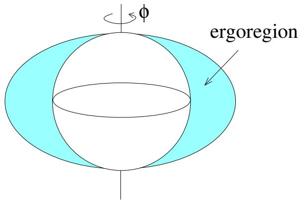
Figure 45. The ergoregion outside the Kerr black hole.

To see this, we look at the norm of $K$ ,

$$g_{\mu \nu }{K}^{\mu }{K}^{\nu }=g_{tt}=-\frac{1}{{\rho }^2}\left(r^2-2GMr+a^2{\cos }^2\theta \right)$$

This is negative, and hence K is timelike, for large r. However, K becomes null when

$$r^2-2GMr-a^2{\cos }^2\theta =0\Rightarrow r=GM\pm \sqrt{G^2{M}^2-a^2{\cos }^2\theta }\text{\hspace{1em}(6.30)}$$

We should compare this to the horizons, which sit at $r_{\pm }=GM\pm \sqrt{G^2{M}^2-a^2}$ . The smaller root in (6.30) sits inside the horizon, but the larger root sits outside the horizon, except at the poles $\theta =0,\pi$ where it touches. We learn that K becomes spacelike in a region outside the horizon,

$$GM+\sqrt{G^2{M}^2-a^2}<r<GM+\sqrt{G^2{M}^2-a^2{\cos }^2\theta }$$

This is called the ergoregion. It is sketched in Figure 45. The outer boundary of the ergoregion is called the ergosurface.

Inside the ergoregion, an observer cannot follow integral curves of K because these curves are no longer timelike. This means that, no matter how hard you fire your rocket thrusters, you cannot sit at constant $r,\theta$ and $\varphi .$ . To see what’s happening, let’s look again at the Kerr metric

$$d{s}^2=-\frac{\Delta }{{\rho }^2}{\left(dt-a{\sin }^2\theta d\varphi \right)}^2+\frac{{\sin }^2\theta }{{\rho }^2}{\left[(r^2+a^2)d\varphi -adt\right]}^2+\frac{{\rho }^2}{\Delta }d{r}^2+{\rho }^{2}d{\theta }^2$$

We want to find a timelike curve, with $d{s}^2<0$ . Moving in the r and θ directions do not help, since $g_{rr}$ and $g_{\theta \theta }$ are both positive. In fact, the only negative term comes from $g_{t\varphi }$ . This means that any timelike trajectory in the ergoregion necessarily requires movement in $\varphi .$

This is an example of frame dragging, albeit an extreme one. In the ergoregion, observers are necessarily swept around by the rotation of the black hole. They can still escape the black hole’s clutches should they wish, since they have not yet crossed the outer horizon, but as long as they remain in ergoregion they rotate relative to asymptotic observers.

The Penrose Process

A clever idea, due to Penrose, allows us to extract energy from a rotating black hole. To motive this, consider again the Killing vector $K={\partial }_t$ . As we explained in Section 4.3.2, we can use K to assign an energy to any observer with 4-momentum $P^{\mu }$ 2

$$E=-K_{\mu }{P}^{\mu }$$

The 4-momentum is necessarily timelike. If K is also timelike, then the negative sign in the definition above ensures that E is positive. This is because the inner product of two timelike vectors is always negative. However, in the ergoregion K is spacelike, so it is possible for the energy to be negative.

Here, then, is the mechanism to extract energy from a black hole. We send in an object along a geodesic, with 4-momentum $P^{\mu }$ . Because it travels along a geodesic, the energy $E=-K\cdot P$ is conserved and so remains positive even when the object enters the ergoregion.

Once in the ergoregion, we arrange for the object to split into two. (In terms of particle physics, you could imagine a particle decaying although it’s rather harder to arrange the details of this before hand.) Conservation of energy and momentum require

$$P=P_1+P_2$$

and, correspondingly,

$$E=E_1+E_2$$

But inside the ergoregion, it is possible to arrange things so that $E_1<0$ . Clearly we must then have $E_2>0$ . Each of these smaller objects then follows their own geodesic. Because $E_1<0$ it is not possible for the first particle to escape the ergoregion; typically, it will instead fall into the black hole. However, there is no such restriction on the second particle with $E_2$ and it is possible to arrange things so that this escapes the black hole and comes back to the asymptotic region, now with $E_2>E$ . In other words, the object returns with more energy than it started.

Extracting energy from the black hole means that its mass decreases. (This backreaction is not included in the calculation above which is done in a fixed background.) If you decrease the mass sufficiently, you might wonder if you can violate the extremality bound to get $J>G{M}^2$ , revealing a naked singularity. Fortunately, this can’t happen: a decrease of the mass must be accompanied by a corresponding decrease in the angular momentum.

To see this, consider the combination of Killing vectors

$$\xi =K+\Omega L=\frac{\partial }{\partial t}+\Omega \frac{\partial }{\partial \varphi }\text{\hspace{1em}(6.31)}$$

This is also a Killing vector for any constant $\Omega .$ We know that K is mostly spacelike on the horizon $r=r_{+}$ . (The exception is at $\theta =0,\pi$ where the horizon intercepts the ergosurface so K is null.) The angular momentum vector $L$ is also spacelike on the horizon. However, there is a special choice of $\Omega$ so that $\xi$ becomes null everywhere on the horizon.

To see this, note that the norm of $\xi$ is

$${\xi }^2=g_{tt}+2\Omega g_{t\varphi }+{\Omega }^2{g}_{\varphi \varphi }$$

We can make ${\xi }^2=0$ at a general r and θ by taking

$$\Omega (r,\theta )=\frac{-g_{t\varphi }\pm \sqrt{g_{t\varphi }^2-g_{tt}{g}_{\varphi \varphi }}}{g_{\varphi \varphi }}$$

If we restrict to the horizon, $r=r_{+}$ then $\Delta =0$ and the identity (6.28) tells us that $g_{t\varphi }^2=g_{tt}{g}_{\varphi \varphi }$ , and we get $\Omega =-g_{t\varphi }/g_{\varphi \varphi }$ . A quick look at the metric (6.27) then shows us that the $\theta$ dependence drops out, leaving us with the constant

$$\Omega =\frac{a}{r_{+}^2+a^2}$$

With this choice of $\Omega ,$ the Killing vector $\xi$ generates null geodesics on the horizon. The frame dragging now means that these geodesics necessarily rotate in the $\varphi$ direction. We interpret $\Omega$ as the angular velocity of the black hole.

We can use $\xi$ to place a restriction on the amount of energy that can be extracted by the Penrose process. The Killing vector $\xi$ is future-pointing, which means that, for any 4-momentum $P_{-}$

$${\xi }_{\mu }{P}^{\mu }\le 0\Rightarrow -E+\Omega j\le 0$$

where $j=L_{\mu }{P}^{\mu }$ is the angular momentum of the particle. Applying this to the particle with $E_1<0$ that falls into the black hole, we have

$$E_1\ge \Omega j_1\text{\hspace{1em}(6.32)}$$

In this sense, we necessarily extract more angular momentum than energy from the black hole. To see that this bound does indeed prohibit the formation of super-extremal rotating black holes, consider the following combination

$$A=8\pi \left[G^2{M}^2+G\sqrt{G^2{M}^4-J^2}\right]=8\pi GM\left[GM+\sqrt{G^2{M}^2-a^2}\right]$$

If the black hole loses both mass δM and angular momentum $\delta J$ , the quantity A changes as

$$\frac{\delta A}{16\pi }=G^{2}M\delta M+\frac{G^3{M}^3\delta M-\frac{1}{2}GJ\delta J}{\sqrt{G^2{M}^4-J^2}}=\frac{GJ}{2\sqrt{G^2{M}^4-J^2}}\left[\frac{\delta M}{\Omega }-\delta J\right]$$

where, in the second equality, we’ve used the expression $r_{+}=GM+\sqrt{G^2{M}^2-a^2}$ 2 which means that $r_{+}^2+a^2=2GM(GM+\sqrt{G^2{M}^2-a^2})$ . A few lines of algebra then gives the result.

The particle plunging beyond the event horizon results in a reduction of the mass $\delta M=E_1$ of the black hole and a change in the angular momentum $\delta J=j_1$ . The inequality (6.32) tells us that $\delta M\ge \Omega \delta J$ and so

$$\delta A\ge 0$$

In other words, A is a quantity which is monotonically increasing in the Penrose process. In particular, this ensures that it’s not possible to turn a sub-extremal Kerr black hole into a super-extremal black hole with a naked singularity through the Penrose process.

A Hint of the Area Theorem

The quantity A has a rather special geometric meaning: it is the area of the event horizon of the black hole

$$A={\int }_0^{\pi }d\theta {\int }_0^{2\pi }d\varphi {\sqrt{g_{\theta \theta }{g}_{\varphi \varphi }}|}_{r=r_{+}}=4\pi (r_{+}^2+a^2)=8\pi \left[G^2{M}^2+G\sqrt{G^2{M}^4-J^2}\right]$$

where we have evaluated the integral at $r=r_{+}$ , which means that $\Delta =0$ . Our analysis above shows that the area of the black hole always increases.

This is a baby version of a much deeper theorem, proved by Hawking, which says that the area of a black hole increases under all physical processes. Indeed, there is a deep reason behind this: the area of the black hole has the interpretation of entropy, through the famous Bekenstein-Hawking formula

$$S_{BH}=\frac{c^{3}A}{4G\hslash }$$

The fact that the area necessarily increases is then part of the generalised second law of thermodynamics.

Superradiance

There is a grown-up version of the Penrose process in which fields scatter of a Kerr black hole, and return amplified. This effect is known as superradiance.

Here we sketch this phenomenon for a massless scalar field Φ. The energy-momentum tensor is (4.51)

$$T_{\mu \nu }={\nabla }_{\mu }\Phi {\nabla }_{\nu }\Phi -\frac{1}{2}{g}_{\mu \nu }{\nabla }^{\rho }\Phi {\nabla }_{\rho }\Phi$$

We know from Section 4.5.5 that we can form a conserved current by contracting $T^{\mu \nu }$ with a suitable Killing vector. In particular, we can measure energy by contracting with $K={\partial }_t$ to give the current

$$J^{\nu }=-K_{\mu }{T}^{\mu \nu }=-(K^{\mu }{\nabla }_{\mu }\Phi ){\nabla }^{\nu }\Phi +\frac{1}{2}({\nabla }^{\rho }\Phi {\nabla }_{\rho }\Phi )K^{\nu }$$

This obeys ${\nabla }_{\mu }{J}^{\mu }=0$

We now repeat the kind of calculation that we saw in Section 4.5.5. The energy in the field on a spatial hypersurface outside the black hole is

$$E(\Sigma )={\int }_{\Sigma }{d}^{3}x\sqrt{\gamma }{n}_{\mu }{J}^{\mu }$$

with ${\gamma }_{ij}$ the pull-back of the metric onto $\Sigma .$ , and $n^{\mu }$ the future-pointing normal. We now integrate ${\nabla }_{\mu }{J}^{\mu }$ over the shaded region in Figure 46. Assuming that $\nabla \Phi =0$ at spatial infinity, $i^0$ , we have

$$0={\int }_V{d}^{4}x\sqrt{-g}{\nabla }_{\mu }{J}^{\mu }={\int }_{{\Sigma }_2}{d}^{3}x\sqrt{{\gamma }_2}{n}_{\mu }^2{J}^{\mu }-{\int }_{{\Sigma }_1}{d}^{3}x\sqrt{{\gamma }_1}{n}_{\mu }^1{J}^{\mu }+{\int }_{\mathcal{N}}{d}^3{S}_{\mu }{J}^{\mu }$$

with $\mathcal{N}$ the appropriate part of the horizon. Rearranging, we have

$$E({\Sigma }_2)-E({\Sigma }_1)=-\int d^{2}Adv{\xi }_{\mu }{J}^{\mu }$$

where v is the null Kerr coordinate, $\xi$ is the null Killing vector (6.31) along the horizon, and $d^{2}A$ is the spatial cross-section of the horizon.

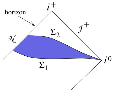
Figure 46. Integrating over a spatial region outside a black hole.

The power absorbed by the black hole per unit null time is then

$$\mathcal{P}=-\int d^{2}A{\xi }_{\mu }{J}^{\mu }$$

with

$${\xi }_{\mu }{J}^{\mu }=-(K^{\mu }{\nabla }_{\mu }\Phi )({\xi }^{\nu }{\nabla }_{\nu }\Phi )+\frac{1}{2}({\nabla }^{\rho }\Phi {\nabla }_{\rho }\Phi )({\xi }_{\mu }{K}^{\mu })$$

The final term vanishes because, when evaluated on the horizon, $\xi \cdot K=0$ . To see this, we evaluate

$${\xi }_{\mu }{K}^{\mu }=g_{tt}+\Omega g_{t\varphi }\Rightarrow {{\xi }_{\mu }{K}^{\mu }|}_{r_{+}}={\left(g_{tt}-\frac{g_{t\varphi }^2}{g_{\varphi \varphi }}\right)}_{r=r_{+}}$$

But evaluated on the horizon, where $\Delta =0$ , the identity (6.28), tells us that $g_{t\varphi }^2=g_{tt}{g}_{\varphi \varphi }$ and so ${\xi }_{\mu }{K}^{\mu }=0$ . This means that we can write the power as

$$\mathcal{P}=\int d^{2}A(K^{\mu }{\nabla }_{\mu }\Phi )({\xi }^{\nu }{\nabla }_{\nu }\Phi )=\int d^{2}A\frac{\partial \Phi }{\partial v}\left(\frac{\partial \Phi }{\partial v}+\Omega \frac{\partial \Phi }{\partial \chi }\right)$$

We can expand the scalar field in angular momentum modes. In terms of the Kerr coordinates (6.29),

$$\Phi ={\Phi }_0(r,\theta )\cos (\omega v+\nu \chi )$$

We take the frequency to be positive: $\omega >0$ . Periodicity of $\chi$ requires that the angular momentum is quantised, with $\nu \in \mathbf{Z}$ . The time averaged power absorbed by the black hole is

$$\bar{\mathcal{P}}=\frac{1}{2}\left[\int d^{2}A{\Phi }_0^2(r_{+},\theta )\right]\omega (\omega -\Omega \nu )$$

For high frequency waves, this power is always positive, telling us that the black hole absorbs energy as expected. However, for frequencies small compared to the angular momentum of the ingoing wave,

$$\omega <\Omega \nu$$

the power absorbed is negative. This is the field theoretic version of the Penrose process.

6.3.4 The No Hair Theorem

Uniqueness theorems tell us that the Kerr metric is the most general black hole solution to the vacuum Einstein equations. But what if we add further fields to the action?

We’ve already seen in Section 6.2 that adding a Maxwell field to the action opens up a new possibility: a black hole solution that carries electric or magnetic charge. There is a generalisation that describes a black hole with both charge and rotation. This amalgam of the Reissner-Nordstr¨om and Kerr solutions has metric

$$\begin{array}{rl}& d{s}^2=-\left(1-\frac{2GMr}{{\rho }^2}+\frac{e^2}{{\rho }^2}\right)d{t}^2-\frac{2a{\sin }^2\theta }{{\rho }^2}\left[2GMr-e^2\right]dtd\varphi +\frac{{\rho }^2}{\Delta }d{r}^2\\ & +\frac{{\sin }^2\theta }{{\rho }^2}\left[(r^2+a^2{)}^2-\Delta a^2{\sin }^2\theta \right]d{\varphi }^2+{\rho }^{2}d{\theta }^2\end{array}$$

where $\Delta (r)$ and ${\rho }^2(r,\theta )$ now take the form

$$\Delta =r^2-2GMr+a^2+e^2$$

$${\rho }^2=r^2+a^2{\cos }^2\theta$$

$$e^2=\frac{G}{4\pi }\sqrt{Q_e^2+Q_m^2}$$

Meanwhile, the gauge field is given by

$$A=-\frac{Q_{e}r}{4\pi {\rho }^2}(dt-a{\sin }^2\theta d\varphi )-\frac{Q_m\cos \theta }{4\pi {\rho }^2}(adt-(r^2+a^2)d\varphi )$$

This is the Kerr-Newman solution.

This is the most general black hole solution of the Einstein-Maxwell equations: the black holes are characterised by mass, M, angular momentum J, and electric and magnetic charges $Q_e$ and $Q_m$ . Note that all of these are familiar conserved quantities of classical systems.

What about other fields? It turns out that these cannot take on other time-independent profiles in the presence of a black hole. This is known as the no hair theorem. (It is a statement about black holes in asymptotically flat spacetimes; the story is different for black holes in AdS.)

Here we sketch the no hair theorem for a free, massive scalar field Φ. The fact that we’re looking for time-independent solutions means that

$$K^{\mu }{\nabla }_{\mu }\Phi =0\text{\hspace{1em}(6.33)}$$

where $K^{\mu }$ is a Killing vector that is timelike outside the horizon. (It is $K={\partial }_t$ in the usual coordinates.) The action for the scalar field is

$$\begin{array}{rl}& S_{\mathrm{scalar}}=\int d^{4}x\sqrt{-g}\frac{1}{2}\left(-g^{\mu \nu }{\nabla }_{\mu }\Phi {\nabla }_{\nu }\Phi -m^2{\Phi }^2\right)\\ & =\int d^{4}x\sqrt{-g}\frac{1}{2}\left(-g^{tt}{\partial }_t\Phi {\partial }_t\Phi -2g^{ti}{\partial }_t\Phi {\partial }_i\Phi -g^{ij}{\partial }_i\Phi {\partial }_j\Phi -m^2{\Phi }^2\right)\end{array}$$

The fact that we are working in a mixed-signature metric means that the gradient terms come with a mix of signs. However, restricting to time independent configurations (6.33) means that the time derivatives vanish and so $g^{\mu \nu }{\nabla }_{\mu }\Phi {\nabla }_{\nu }\Phi \ge 0$ . In particular, this means that the action is the sum of two terms, each of which is non-positive.

The proof of the no hair theorem in this case proceeds in a similar way to our demonstration of superradiance. We integrate over the spacetime region V outside a black hole, as shown in Figure 46. This region is bounded by two spatial hypersurfaces, ${\Sigma }_1$ and ${\Sigma }_2$ , with normal $n^{\mu }\sim K^{\mu }$ , the horizon and an asymptotic region. Integrating by parts we have

$$S_{\mathrm{scalar}}={\int }_V{d}^{4}x\sqrt{-g}\frac{1}{2}\Phi \left(+g^{\mu \nu }{\nabla }_{\mu }{\nabla }_{\nu }\Phi -m^2\Phi \right)-{\int }_{\partial V}{d}^{3}x\sqrt{-\gamma }{n}^{\mu }\Phi {\nabla }_{\mu }\Phi$$

The first, bulk, term vanishes for any Φ that solves the equation of motion. That leaves the second, boundary, term. This vanishes on the two spatial hypersurfaces by dint of (6.33). It also vanishes on the horizon for the same reason, since the normal to the horizon is $K^{\mu }$ the timelike Kiling vector. That just leaves the asymptotic region. For asymptotically flat spacetimes, it’s not too hard to show that $\Phi \sim 1/r$ as $r\to \infty$ 2 which is fast enough to ensure that there’s no contribution from infinity.

The upshot of this argument is that, when evaluated on a time-independent solution to the equation of motion, we have $S_{\mathrm{scalar}}=0$ when integrated over any region V of a black hole spacetime. Furthermore, $S_{\mathrm{scalar}}$ is the sum of two non-positive terms, so each of these terms must individually vanish. When $m\ne 0$ , we have $m^2{\Phi }^2=0$ so the only solution is the trivial one $\Phi =0$ . (When $m^2=0$ , we have ${\partial }_i\Phi =0$ , so any $\Phi =$ constant is allowed.) This is the no hair theorem: the field $\Phi$ cannot develop a static profile in the presence of a black hole.

来源与版本

正文：英文 · OCR 机器稿 · 待校对

核对状态：OCR 机器稿 · 待校对

原书 PDF

来源版本：michaelmas-2019-source-20260923

来源 PDF SHA-256：3ba65dc61f22a69c7d5fdf3e8e1f641efbfa6cf49a44b3dcb0fd5367ba9fcf1c

OCR 来源 SHA-256：5bbc97c50eaf0b03554f3ef1174075158c1598ac18f79242ddcda9dd2f12f618

OCR 产物 SHA-256：d148a20fcc2bf788e8f4d16468220df88384ed4e822ffb9e6da1853916a38a7a