6.2 Charged Black Holes

In this section, we describe a solution to the Einstein-Maxwell equation corresponding to a black hole carrying electric or magnetic charge.

Black holes with large amounts of electric charge do not arise in Nature. (Such black holes would attract the opposite charge and neutralise.) Nonetheless, there are a number of theoretical reasons for studying these black holes. In particular, charged black holes exhibit a rather different causal structure from the Schwarzschild solution and, for our purposes, this will provide a warm-up for the rotating black holes that we will study in Section 6.3. Moving beyond these lectures, it turns out that charged black holes provide a laboratory in which we can address certain questions about the quantum make-up of black holes.

6.2.1 The Reissner-Nordstr¨om Solution

Charged black holes arise as a solution to Einstein-Maxwell theory, with action

$$S=\int d^{4}x\sqrt{-g}\left[\frac{1}{16\pi G}R-\frac{1}{4}{F}^{\mu \nu }{F}_{\mu \nu }\right]\text{\hspace{1em}(6.19)}$$

The equations of motion are the Maxwell equation

$${\nabla }^{\mu }{F}_{\mu \nu }=0$$

together with the Einstein-Maxwell equation

$$R_{\mu \nu }-\frac{1}{2}R{g}_{\mu \nu }=8\pi G\left(F_{\mu }^{\rho }{F}_{\nu \rho }-\frac{1}{4}{g}_{\mu \nu }{F}^{\rho \sigma }{F}_{\rho \sigma }\right)$$

where the right-hand side is the Maxwell stress-energy tensor that we calculated in (4.52).

These equations of motion admit a spherically symmetric solution with gauge field

$$A=-\frac{Q_e}{4\pi r}dt-\frac{Q_m}{4\pi }\cos \theta d\varphi$$

The metric takes the familiar spherically symmetric form

$$d{s}^2=-f(r{)}^{2}d{t}^2+f(r{)}^{-2}d{r}^2+r^{2}d{\Omega }_2^2$$

where, this time,

$$f(r{)}^2=1-\frac{2GM}{r}+\frac{e^2}{r^2}\mathrm{with}{e}^2=\frac{G}{4\pi }(Q_e^2+Q_m^2)$$

This is the Reissner-Nordstr¨om solution, discovered over a period of years from 1916 to 1921.

An analog of Birkhoff’s theorem says that the Reissner-Nordstr¨om solution is almost the unique spherically symmetric solution of the Einstein-Maxwell equations. There is one exception: there is a solution with geometry ${\mathrm{AdS}}_2\times {\mathbf{S}}^2$ , threaded with electric flux; we’ll see how this emerges a special limit of the Reissner-Nordstr¨om solution in Section 6.2.5.

The dt term in the gauge field describes a radial electric field. Meanwhile, the dϕ term is the gauge field for a magnetic monopole; it is only rotationally invariant up to a gauge transformation. (See, for example, the lectures on Gauge Theory for more discussion.) Both of these charges can be measured asympotically as explained in 3.2.5. One can check that

$$Q_e={\int }_{{\mathbf{S}}^2}\star F\text{ and }{Q}_m={\int }_{{\mathbf{S}}^2}F$$

The solution has non-vanishing electric and magnetic charge, even though the theory (6.19) has no charge matter. The electric and magnetic charges can be viewed as lurking in the singularity.

To get some intuition for the Reissner-Nordstr¨om black hole, we write the metric factor as

$$f(r{)}^2=\frac{1}{r^2}(r-r_{+})(r-r_{-})$$

Here the two roots are given by

$$r_{\pm }=GM\pm \sqrt{G^2{M}^2-e^2}\text{\hspace{1em}(6.20)}$$

In the limit where $e\to 0$ , the smaller root merges with the singularity, $r_{-}\to 0$ while the larger root coincides with the Schwarzschild radius $r_{+}\to 2GM$ . The physical interpretation of the metric depends on the roots of this polynomial. We deal with these cases in turn.

6.2.2 Super-Extremal Black Holes

Super-extremal black holes have $|e|>GM$ . This means that $f(r{)}^2$ has no zero, and so the metric has no horizon. This situation is analogous to the negative mass Schwarzschild solution. It has a naked singularity. It is unphysical.

If we take, for example, an electrically charged black hole, the super-extremal condition $e^2>G^2{M}^2$ translates to the requirement that $Q_e^2/4\pi >G{M}^2$ . But this ensures that the electromagnetic repulsion between two such black holes beats the gravitational attraction. For this reason, it is hard to see how such objects could form in the first place.

Of course, all charged sub-atomic particles are super-extremal in the sense that the electrical repulsion beats the gravitational attraction. There is no contradiction here: sub-atomic particles simply are not black holes! For example, a particle with mass m has Compton wavelength $\lambda =\hslash /2\pi mc$ . (For once we’ve put the factor of c back in this equation.) The requirement that the Compton wavelength is always larger than the Schwarzschild radius is

$$\frac{\hslash }{2\pi mc}>\frac{2Gm}{c^2}\Rightarrow m^2<\frac{\hslash c}{4\pi G}=2M_{\mathrm{pl}}^2$$

This conclusion should not be surprising: it tells us that quantum effects are more important than gravitational effects for any sub-atomic particle that weighs less than the Planck mass, which itself is a whopping $10^{18}\mathrm{GeV}$ . This is roughly the mass of a grain of sand.

6.2.3 Sub-Extremal Black Holes

Reissner-Nordstr¨om black holes with $|e|<GM$ are called sub-extremal. These are the physically relevant solutions.

There are now two roots, $r_{\pm }$ , of the metric function $f(r{)}^2$ . The Kretschmann scalar diverges at neither of these roots, suggesting that both are horizons. So charged black holes have two horizons: an outer one at $r_{+}$ and an inner one at $r_{-}$

The presence of two roots changes the role played by the singularity. This is because the $g_{rr}$ metric component flips sign twice so that r is again a spatial coordinate by the time we get to $r<r_{-}$ ₋. This suggests that $r=0$ is now a timelike singularity, as opposed to the spacelike singularity that we saw in the Schwarzschild case. The purpose of this section is to understand these points in some detail.

We will follow the same path that we took to understand the Schwarzschild solution. We start by introducing a tortoise coordinate, analogous to (6.6), now defined by

$$d{r}_{\star }^2=\frac{1}{f(r{)}^4}d{r}^2$$

The solution to this differential equation is

$$r_{\star }=r+\frac{1}{2{\kappa }_{+}}\log \left|\frac{r-r_{+}}{r_{+}}\right|+\frac{1}{2{\kappa }_{-}}\log \left|\frac{r-r_{-}}{r_{-}}\right|\text{\hspace{1em}(6.21)}$$

with

$${\kappa }_{\pm }=\frac{r_{\pm }-r_{\mp }}{2r_{\pm }^2}$$

We will see later that ${\kappa }_{\pm }$ have the interpretation of the surface gravity on the two horizons.

The tortoise coordinate $r_{\star }$ takes values in $r_{\star }\in (-\infty ,+\infty )$ as $r\in \mathsf{\Gamma }(r_{+},\infty )$ . We introduce a pair of null coordinates, just as for the Schwarzschild black hole

$$v=t+r_{\star }\mathrm{and}u=t-r_{\star }$$

Exchanging $t$ in favour of the null coordinate $v,$ we get the Reissner-Nordstr¨om black hole in ingoing Eddington-Finkelstein coordinates

$$d{s}^2=-f(r{)}^{2}d{v}^2+2dvdr+r^{2}d{\Omega }_2^2\text{\hspace{1em}(6.22)}$$

This metric is smooth for all $r>0$ , and has a coordinate singularity at $r=0$ . This ensures that we can extend the Reissner-Nordstr¨om black hole to all $r>0$ . The same kind of arguments that we used for the Schwarzschild black hole again tell us that $r=r_{+}$ is a null surface, and no signal from $r<r_{+}$ can reach ${\mathcal{I}}^{+}$ . In other words, $r=r_{+}$ is a future event horizon.

Similarly, we could extend the Reissner-Nordstr¨om solution using outgoing Eddington-Finkelstein coordinates, to reveal a white hole region.

Kruskal Spacetime

We have still to understand the role played by the inner horizon at $r=r.$ ₋ and, relatedly, the global structure of the spacetime. To make progress, we introduce two different kinds of Kruskal-like coordinates

$$U_{\pm }=-e^{-{\kappa }_{\pm }u}\mathrm{and}{V}_{\pm }=\pm e^{{\kappa }_{\pm }v}\text{\hspace{1em}(6.23)}$$

In the limit $e\to 0$ , we have ${\kappa }_{+}\to 4GM$ and the coordiantes $U_{+}$ and $V_{+}$ coincide with the Kruskal-Szekeres coordinates (6.12).

To start, we work with the coordinates $U_{+}$ and $V_{+}$ . These null coordinates have the property that

$$U_{+}{V}_{+}=-e^{2{\kappa }_{+}{r}_{\star }}=-\left(\frac{r-r_{+}}{r_{+}}\right){\left(\frac{r_{-}}{r-r_{-}}\right)}^{r_{-}^2/r_{+}^2}{e}^{2{\kappa }_{+}r}\text{\hspace{1em}(6.24)}$$

The Reissner-Nordstr¨om metric is now,

$$\begin{array}{rl}& d{s}^2=-f(r{)}^{2}dudv+r^{2}d{\Omega }_2^2\\ & =-\frac{r_{+}{r}_{-}}{{\kappa }_{+}^2{r}^2}{\left(\frac{r-r_{-}}{r_{-}}\right)}^{1+r_{-}^2/r_{+}^2}{e}^{-2{\kappa }_{+}r}d{U}_{+}d{V}_{+}+r^{2}d{\Omega }_2^2\end{array}$$

where, as usual, we should now view $r=r(U_{+},V_{+})$ , this time using (6.24). The metric has started to get a little ugly, but the exact form won’t bother us. More interesting is what the various regimes of $U_{+}$ and $V_{+}$ coordinates correspond to.

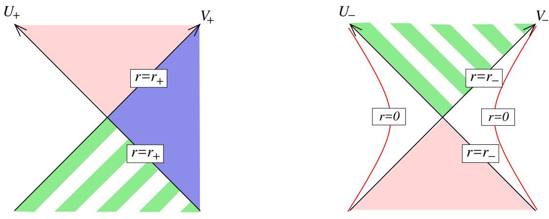
Figure 40.

The exterior of the Reissner-Nordstr¨om black hole is the region $r>r_{+}$ . From (6.23) and (6.24), we see that this corresponds to $U_{+}<0$ and $V_{+}>0$ . But, just as for the Schwarzschild-Kruskal spacetime, we can now extend the Kruskal coordinates to $U_{+},V_{+}\in \mathbf{R}$ . This gives the now-familiar spacetime diagram, split into four quadrants depending on the sign of $U_{+}$ and $V_{+}$ . This is shown in the left-hand diagram of Figure $40;$ the region outside the horizon is the right-hand quadrant and is shaded blue; the region $r_{-}<r<r_{+}$ is the upper quadrant and is shaded pink.

At this point, however, the story diverges from that of Schwarzschild. This is because the Kruskal-type coordinates $U_{+}$ and $V_{+}$ do not extend down to the singularity at $r=0$ Instead, from (6.24), we see that as $r\to r.$ , we have $U_{+}{V}_{+}\to \infty$ . This means that the coordinates $U_{+}$ and $V_{+}$ only extend down to the inner horizon $r=r_{-}$

There was no such obstacle in the Eddington-Finkelstein coordinates (6.22), which happily extended down to the singularity at $r=0$ . This means that the Kruskal coordinates $U_{+}$ and $V_{+}$ are not the final extension: we can do better.

This is where the other coordinates $U_{-}$ and $V_{-}$ in (6.23) come in. The regime between the horizons with $r_{-}<r<r_{+}$ (in ingoing Eddington-Finkelstein coordinates) corresponds to $U_{-},V_{-}<0$ . We then have

$$U_{-}{V}_{-}=e^{2{\kappa }_{-}{r}_{\star }}=\left(\frac{r-r_{-}}{r_{-}}\right){\left(\frac{r_{+}}{r_{+}-r}\right)}^{r_{+}^2/r_{-}^2}{e}^{2{\kappa }_{-}r}$$

These coordinates have the property that $U_{-}{V}_{-}\to \infty$ as $r\to r_{+}$ from below. In other words, they cover the region inside the black hole, but not outside. We can now extend the $U_{-},V_{-}$ coordinates, as shown in the right-hand diagram of Figure 40, where the lower-most quadrant is shaded pink, to show that it should be identified with the upper-most quadrant of the first figure.

The $U_{-},V_{-}$ coordinates cover the singularity at $r=0$ . In fact, there are two such singularities, one in each of the left and right-quadrants as shown as red lines in the figure. Spacetime does not extend beyond the singularity. Importantly, and in contrast to the Schwarzschild black hole, the singularities are timelike. This is the kind of singularity that you might have imagined black holes to have: it is like the worldline of a particle. However, this means that there is nothing inevitable about the singularity of the Reissner-Nordstr¨om black hole: there exist timelike worldlines that a test particle could follow that miss the singularity completely.

Such fortunate worldliners will ultimately end up in the upper-most quadrant of the right-hand diagram of Figure 40, where $U_{-},V_{-}>0$ . This is a new, unanticipated part of spacetime. One finds that geodesics hit the boundary of this region at a finite value of the affine parameter. This means that our spacetime must be extended yet further! In fact, the upper-most region of the right-hand diagram is isomorphic to the lowermost region of the left-hand diagram. These regions are shaded in the same colour, but with different stripes to show that the metrics are isomorphic, but they should not be identified. (Doing so would lead to a closed timelike curve.) Instead, we introduce yet a third set of coordinates, $U_{+}^{\prime }$ and $V_{+}^{\prime }$ . This gives rise to a new part of spacetime, isomorphic to the left-hand diagram. The whole procedure then repeats ad infinitum.

The Kruskal diagrams can be patched together to give the Penrose diagram for the Reissner-Nordstr¨om black hole. Perhaps surprisingly, it is an infinitely repeating pattern, both to the past and to the future, as shown in Figure 41, where the conformal factor has been chosen so the singularity appears as a vertical line.

6.2.4 Cauchy Horizons: Strong Cosmic Censorship

The Penrose diagram reveals the meaning of the inner horizon $r=r_{-}$ . Consider some initial data specified on a spatial surface Σ, like that shown in Figure 42. Such a surface is referred to as as Cauchy surface. We then evolve this initial data forward using the equations of motion.

Sadly, once we encounter a timelike singularity, such evolution is no longer possible, because we need information about what the fields are doing at the singularity. We see that the data on $\Sigma$ can only be evolved as far as the inner horizon $r=r.$ . The null surface $r=r.$ ₋ is called a Cauchy horizon.

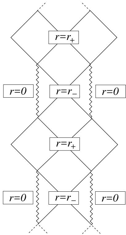
Figure 41. The Penrose diagram for the Reissner-Nordstr¨om black hole.

The Cauchy horizon is believed to be unstable. To get some intuition for this, consider the two observers shown in Figure 42. Observer A stays sensibly away from the black hole, sending signals with some constant frequency – say, 1 second – into the black hole for all eternity. Meanwhile, adventurous but foolish observer B ventures into the black hole where he receives the signals. But the signals get closer and closer together as he approaches $r=r_{-}$ , an eternities worth of signals arriving in a finite amount of time, like emails on the first day back after vacation. These signals are therefore infinitely blue shifted, meaning that a small perturbation in the asymptotic region results in a divergent perturbation on the Cauchy horizon.

This instability means that much of the Penrose diagram of the Reissner-Nordstr¨om black hole, including the timelike singularity, is unphysical. It is unclear what the end point of the perturbation will be. But, whatever the outcome, you should probably take the Penrose diagram inside the horizon with something of a pinch of salt: if you make it into a black hole interior, your very presence means that it’s very unlikely to look like that depicted in this simple idealised case. One possibility is that the Cauchy horizon $r=r.$ ₋ becomes a singularity.

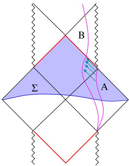
Figure 42. Initial data is specified on $\Sigma .$ , a spatial hypersurface. But this can’t be evolved past the Cauchy horizon, $r=r_{-}$ , shown as the red line in the figure. The extended geometry for the Reissner-Nordstr¨om black hole includes both a future Cauchy horizon, and a past Cauchy horizon.

The instability of the Cauchy horizon is a consequence of a second cosmic censorship conjecture:

The Strong Cosmic Censorship Conjecture: For matter obeying a suitable energy condition, generic initial conditions do not result in a Cauchy horizon. Relatedly, timelike singularities do not form.

Strong cosmic censorship is the statement that general relativity is, generically, a deterministic theory. It is neither stronger nor weaker than weak cosmic censorship and the two, while clearly related, are logically independent. (There is a tradition in general relativity of naming two things “weak” and “strong” even though strong is not stronger than weak.)

6.2.5 Extremal Black Holes

It remains to describe the extremal Reissner-Nordstr¨om black hole, with

$$|e|=GM$$

In this case, the inner and outer horizon coalesce and the metric takes the form

$$d{s}^2=-{\left(1-\frac{GM}{r}\right)}^{2}d{t}^2+{\left(1-\frac{GM}{r}\right)}^{-2}d{r}^2+r^{2}d{\Omega }_2^2\text{\hspace{1em}(6.25)}$$

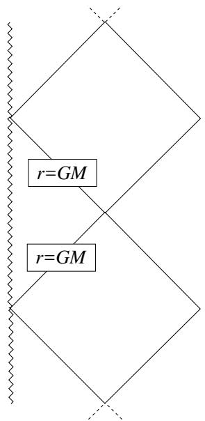
Figure 43. The Penrose diagram for the extremal Reissner-Nordstr¨om black hole.

There is a just a single coordinate singularity at $r=GM$ , but it is now a double pole.

As before, one can use Eddington-Finkelstein coordinates to show that the spacetime can be extended to all $r>0$ , and Kruskal-like coordinates to construct the global causal structure. The resulting penrose diagram is shown in Figure 43.

The extremal black hole has a number of curious features. First, we can look at the spatial distance from a point $r=R$ to the horizon. For a sub-extremal black hole, with an inner and outer horizon, this is given by

$$s={\int }_{r_{+}}^R\frac{dr}{\sqrt{(1-r_{+}/r)(1-r_{-}/r)}}<\infty$$

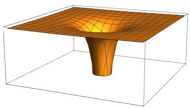
However, for the extremal black hole, with $r_{+}=r_{-}=GM$ , this becomes

$$s={\int }_{GM}^{R}dr{\left(1-\frac{GM}{r}\right)}^{-1}=\infty$$

So the horizon of an extremal black hole lies at infinite spatial distance. In contrast, timelike and null geodesics have no difficulty in reaching the horizon in finite affine parameter.

We should think of the horizon of the black hole as developing an infinite throat as shown in figure; this is what becomes of the Einstein-Rosen bridge, now restricted to just one side.

To understand what the extremal geometry looks like deep within the throat, we can take the near horizon limit. We write

$$r=r_{+}+\eta$$

For $\eta \ll GM$ , the metric (6.25) takes the form

$$d{s}^2=-\frac{{\eta }^2}{r_{+}^2}d{t}^2+r_{+}^2\frac{d{\eta }^2}{{\eta }^2}+r_{+}^{2}d{\Omega }_2^2$$

The first two terms are the metric for the Poincar´e patch of two-dimensional anti-de Sitter spacetime (4.28). The final term is just a two-sphere of constant radius. In this way, we see that the near horizon limit of the extremal Reissner-Nordstr¨om black hole is ${\mathrm{AdS}}_2\times {\mathbf{S}}^2$ ; this is sometimes called the Robinson-Bertotti metric. Similar calculations to this play an important role in motivating the AdS/CFT correspondence from the dynamics of branes in string theory.

Multi-Black Hole Solutions

If we take, for example, electrically charged black holes, the extremality condition $|e|=$ GM means that $Q_e^2/4\pi =G{M}^2$ . Viewed from a somewhat $17^{\mathrm{th}}$ century perspective, this says that the repulsive Coulomb force between two black holes exactly cancels the attractive Newtonian gravitational force. We may then wonder if it’s possible to construct two or more black holes sitting in equilibrium.

The considerations above by no means guarantee the existence of such solutions. It should be clear by now that there’s much more to general relativity than a simple $1/r^2$ Newtonian force law, and we still have the seemingly formidable task of solving the non-linear Einstein equations without the crutch of spherical symmetry. Nonetheless, it’s at least possible that there exist time independent solutions. This is in contrast to Schwarzschild or sub-extremal Reissner-Nordstr¨om black holes, where the attractive force means that two black holes must be orbiting each other, emitting gravitational waves in the process.

Given the complexity of the Einstein equations, it is perhaps surprising that there is not only a time-independent multi-black hole solution, but one that is remarkably simple. To motivate this, we first introduce a new radial coordinate

$$\rho =r-GM$$

Clearly the singularity sits at $\rho =0$ . In this coordinate, the extremal Reissner-Nordstr¨om metric (6.25) takes the form

$$d{s}^2=-H(\rho {)}^{-2}d{t}^2+H(\rho {)}^2\left(d{\rho }^2+{\rho }^{2}d{\Omega }_2^2\right)\mathrm{with}H(\rho )=1+\frac{GM}{\rho }$$

This form now admits a simple generalisation to

$$d{s}^2=-H(\mathbf{x}{)}^{-2}d{t}^2+H(\mathbf{x}{)}^{2}d\mathbf{x}\cdot d\mathbf{x}$$

where x is the usual Cartesian coordinate on ${\mathbf{R}}^3$ . We further make the ansatz for the gauge field $A=H^{-1}dt$ , corresponding to electrically charged black holes. (There is a simple generalisation to black holes carrying both electric and magnetic charge.) Then the non-linear Einstein-Maxwell equations reduce to a very simple linear condition on $H(\mathbf{x})$ ,

$${\nabla }^{2}H=0$$

where ${\nabla }^2$ is the Laplacian on flat ${\mathbf{R}}^3$ . Subject to certain asymptotic boundary conditions this is solved by

$$H(\mathbf{x})=1+\sum _{i=1}^N\frac{1}{|\mathbf{x}-{\mathbf{x}}_i|}$$

This is the Majumdar-Papapetrou solution, discovered in 1947. It describes N black holes sitting at arbitrary positions ${\mathbf{x}}_i$

来源与版本

正文：英文 · OCR 机器稿 · 待校对

核对状态：OCR 机器稿 · 待校对

原书 PDF

来源版本：michaelmas-2019-source-20260923

来源 PDF SHA-256：3ba65dc61f22a69c7d5fdf3e8e1f641efbfa6cf49a44b3dcb0fd5367ba9fcf1c

OCR 来源 SHA-256：5bbc97c50eaf0b03554f3ef1174075158c1598ac18f79242ddcda9dd2f12f618

OCR 产物 SHA-256：978aed2c87d945a31e61a6a61f48492d1b8cbd1d0613bc347c0229449aac993b