5.1 Manifolds

5.1.1 Heuristic introduction

To clarify these points, consider the usual sphere of unit radius in ${\mathbb{R}}^3$ . We parametrize the surface of $S^2$ , among other possibilities, by two coordinate systems—polar coordinates and stereographic coordinates. Polar coordinates $\theta$ and $\varphi$ are usually defined by (figure 5.1)

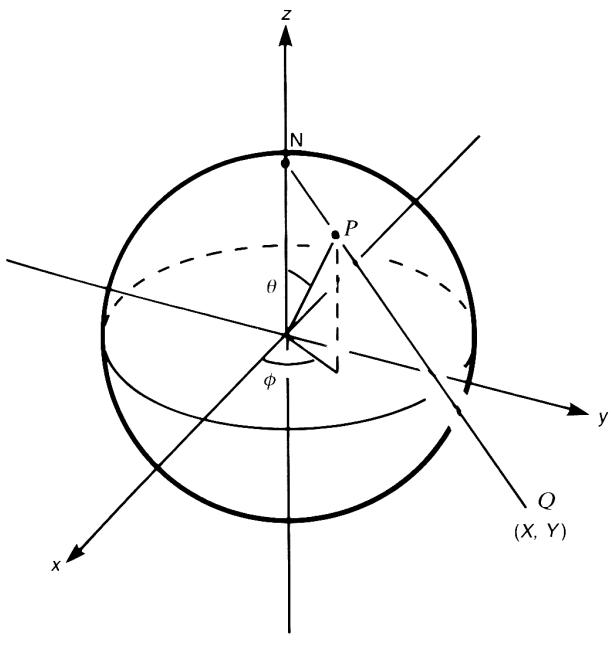
Figure 5.1. Polar coordinates $(\theta ,\varphi )$ and stereographic coordinates $(X,Y)$ of a point $P$ on the sphere $S^2$ .

$$x=\sin \theta \cos \varphi y=\sin \theta \sin \varphi z=\cos \theta ,\text{\hspace{1em}(5.1)}$$

where $\varphi$ runs from 0 to $2\pi$ and $\theta$ from 0 to $\pi$ . They may be inverted on the sphere to yield

$$\theta ={\tan }^{-1}\frac{\sqrt{x^2+y^2}}{z}\varphi ={\tan }^{-1}\frac{y}{x}.\text{\hspace{1em}(5.2)}$$

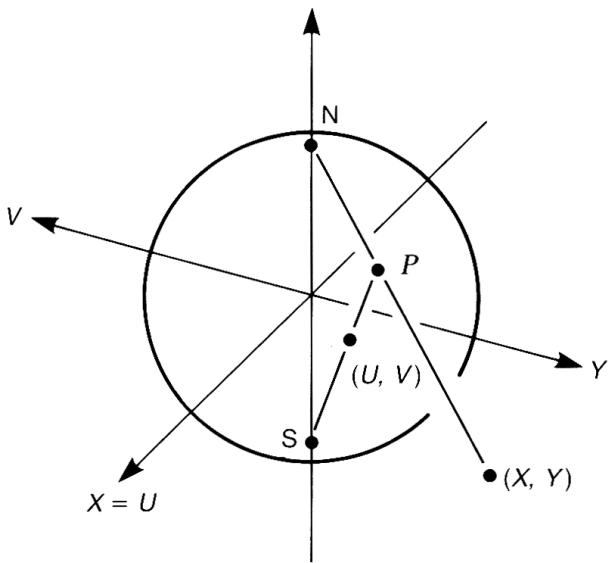
Stereographic coordinates, however, are defined by the projection from the North Pole onto the equatorial plane as in figure 5.1. First, join the North Pole $(0,0,1)$ to the point $P(x,y,z)$ on the sphere and then continue in a straight line to the equatorial plane $z=0$ to intersect at $Q(X,Y,0)$ . Then $X$ and $Y$ are the stereographic coordinates of $P$ . We find

$$X=\frac{x}{1-z}Y=\frac{y}{1-z}.\text{\hspace{1em}(5.3)}$$

The two coordinate systems are related as

$$X=\cot \frac{1}{2}\theta \cos \varphi Y=\cot \frac{1}{2}\theta \sin \varphi .\text{\hspace{1em}(5.4)}$$

Of course, other systems, polar coordinates with different polar axes or projections from different points on $S^2$ , could be used. The coordinates on the sphere may be kept arbitrary until some specific calculation is to be carried out. [The longitude is historically measured from Greenwich. However, there is no reason why it cannot be measured from New York or Kyoto.] This arbitrariness of the coordinate choice underlies the theory of manifolds: all coordinate systems are equally good. It is also in harmony with the basic principle of physics: a physical system behaves in the same way whatever coordinates we use to describe it.

Another point which can be seen from this example is that no coordinate system may be usable everywhere at once. Let us look at the polar coordinates on $S^2$ . Take the equator $(\theta =\frac{1}{2}\pi )$ for definiteness. If we let $\varphi$ range from 0 to $2\pi$ , then it changes continuously as we go round the equator until we get all the way to $\varphi =2\pi$ . There the $\varphi$ -coordinate has a discontinuity from $2\pi$ to 0 and nearby points have quite different $\varphi$ -values. Alternatively we could continue $\varphi$ through $2\pi$ . Then we will encounter another difficulty: at each point we must have infinitely many $\varphi$ -values, differing from one another by an integral multiple of $2\pi$ . A further difficulty arises at the poles, where $\varphi$ is not determined at all. [An explorer on the Pole is in a state of timelessness since time is defined by the longitude.] Stereographic coordinates also have difficulties at the North Pole or at any projection point that is not projected to a point on the equatorial plane; and nearby points close to the Pole have widely different stereographic coordinates.

Thus, we cannot label the points on the sphere with a single coordinate system so that both of the following conditions are satisfied.

(i) Nearby points always have nearby coordinates.
(ii) Every point has unique coordinates.

Note, however, that there are infinitely many ways to introduce coordinates that satisfy these requirements on a part of $S^2$ . We may take advantage of this fact to define coordinates on $S^2$ : introduce two or more overlapping coordinate systems, each covering a part of the sphere whose points are to be labelled so that the following conditions hold.

(i’) Nearby points have nearby coordinates in at least one coordinate system. (ii’) Every point has unique coordinates in each system that contains it.

For example, we may introduce two stereographic coordinates on $S^2$ , one a projection from the North Pole, the other from the South Pole. Are these conditions (i’) and (ii’) enough to develop sensible theories of the manifold? In fact, we need an extra condition on the coordinate systems.

(iii) If two coordinate systems overlap, they are related to each other in a sufficiently smooth way.

Without this condition, a differentiable function in one coordinate system may not be differentiable in the other system.

5.1.2 Definitions

Definition 5.1

$M$ is an $m$ -dimensional differentiable manifold if

(i) $M$ is a topological space;
(ii) $M$ is provided with a family of pairs $\{(U_i,{\phi }_i)\}$ ;
(iii) $\{U_i\}$ is a family of open sets which covers $M$ , that is, ${\cup }_i{U}_i=M$ . ${\phi }_i$ is a homeomorphism from $U_i$ onto an open subset $U_i^{\prime }$ of ${\mathbb{R}}^m$ (figure 5.2); and

Figure 5.2. A homeomorphism ${\phi }_i$ maps $U_i$ onto an open subset $U_i^{\prime }\subset {\mathbb{R}}^m$ , providing coordinates to a point $p\in U_i$ . If $U_i\cap U_j\ne \varnothing$ , the transition from one coordinate system to another is smooth.

(iv) given $U_i$ and $U_j$ such that $U_i\cap U_j\ne \varnothing$ , the map ${\psi }_{ij}={\phi }_i\circ {\phi }_j^{-1}$ from ${\phi }_j(U_i\cap U_j)$ to ${\phi }_i(U_i\cap U_j)$ is infinitely differentiable.

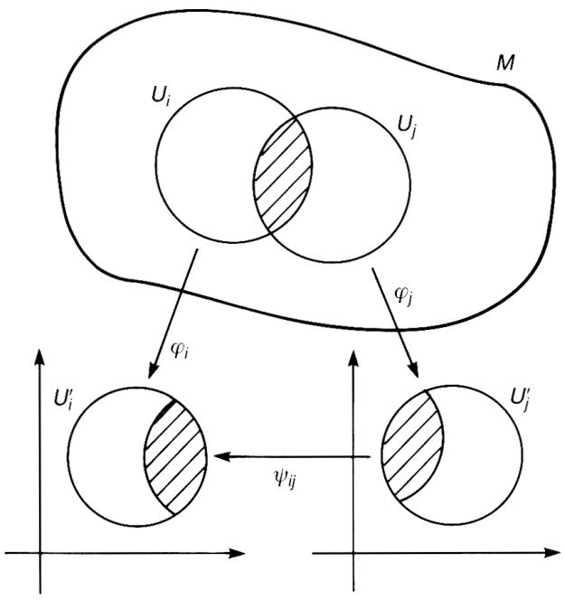
The pair $(U_i,{\phi }_i)$ is called a chart while the whole family $\{(U_i,{\phi }_i)\}$ is called, for obvious reasons, an atlas. The subset $U_i$ is called the coordinate neighbourhood while ${\phi }_i$ is the coordinate function or, simply, the coordinate. The homeomorphism ${\phi }_i$ is represented by $m$ functions $\{x^1(p),\dots ,x^m(p)\}$ . The set $\{x^{\mu }(p)\}$ is also called the coordinate. A point $p\in M$ exists independently of its coordinates; it is up to us how we assign coordinates to a point. We sometimes employ the rather sloppy notation $x$ to denote a point whose coordinates are $\{x^1,\dots ,x^m\}$ , unless several coordinate systems are in use. From (ii) and (iii), $M$ is locally Euclidean. In each coordinate neighbourhood $U_i$ , $M$ looks like an open subset of ${\mathbb{R}}^m$ whose element is $\{x^1,\dots ,x^m\}$ . Note that we do not require that $M$ be ${\mathbb{R}}^m$ globally. We are living on the earth whose surface is $S^2$ , which does not look like ${\mathbb{R}}^2$ globally. However, it looks like an open subset of ${\mathbb{R}}^2$ locally. Who can tell that we live on the sphere by just looking at a map of London, which, of course, looks like a part of ${\mathbb{R}}^2$ ?

If $U_i$ and $U_j$ overlap, two coordinate systems are assigned to a point in $U_i\cap U_j$ . Axiom (iv) asserts that the transition from one coordinate system to another be smooth ( $C^{\infty }$ ). The map ${\phi }_i$ assigns $m$ coordinate values $x^{\mu }$ ( $1\le \mu \le m$ ) to a point $p\in U_i\cap U_j$ , while ${\phi }_j$ assigns $y^{\nu }$ ( $1\le \nu \le m$ ) to the same point and the transition from $y$ to $x$ , $x^{\mu }=x^{\mu }(y)$ , is given by $m$ functions of $m$ variables. The coordinate transformation functions $x^{\mu }=x^{\mu }(y)$ are the explicit form of the map ${\psi }_{ji}={\phi }_j\circ {\phi }_i^{-1}$ . Thus, the differentiability has been defined in the usual sense of calculus: the coordinate transformation is differentiable if each function $x^{\mu }(y)$ is differentiable with respect to each $y^{\nu }$ . We may restrict ourselves to the differentiability up to $k$ th order ( $C^k$ ). However, this does not bring about any interesting conclusions. We simply require, instead, that the coordinate transformations be infinitely differentiable, that is, of class $C^{\infty }$ . Now coordinates have been assigned to $M$ in such a way that if we move over $M$ in whatever fashion, the coordinates we use vary in a smooth manner.

If the union of two atlases $\{(U_i,{\phi }_i)\}$ and $\{(V_j,{\psi }_j)\}$ is again an atlas, these two atlases are said to be compatible. The compatibility is an equivalence relation, the equivalence class of which is called the differentiable structure. It is also said that mutually compatible atlases define the same differentiable structure on $M$ .

Before we give examples, we briefly comment on manifolds with boundaries. So far, we have assumed that the coordinate neighbourhood $U_i$ is homeomorphic to an open set of ${\mathbb{R}}^m$ . In some applications, however, this turns out to be too restrictive and we need to relax this condition. If a topological space $M$ is covered by a family of open sets $\{U_i\}$ each of which is homeomorphic to an open set of $H^m\equiv \{(x^1,\dots ,x^m)\in {\mathbb{R}}^m|x^m\ge 0\}$ , $M$ is said to be a manifold with a boundary, see figure 5.3. The set of points which are mapped to points with $x^m=0$ is called the boundary of $M$ , denoted by $\partial M$ . The coordinates of $\partial M$ may be given by $m-1$ numbers $(x^1,\dots ,x^{m-1},0)$ . Now we have to be careful when we define the smoothness. The map ${\psi }_{ij}:{\phi }_j(U_i\cap U_j)\to {\phi }_i(U_i\cap U_j)$ is defined on an open set of $H^m$ in general, and ${\psi }_{ij}$ is said to be smooth if it is $C^{\infty }$ in an open set of ${\mathbb{R}}^m$ which contains ${\phi }_j(U_i\cap U_j)$ . Readers are encouraged to use their imagination since our definition is in harmony with our intuitive notions about boundaries. For example, the boundary of the solid ball $D^3$ is the sphere $S^2$ and the boundary of the sphere is an empty set.

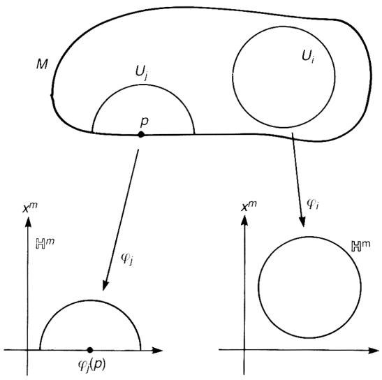
Figure 5.3. A manifold with a boundary. The point $p$ is on the boundary.

5.1.3 Examples

We now give several examples to develop our ideas about manifolds. They are also of great relevance to physics.

Example 5.1

The Euclidean space ${\mathbb{R}}^m$ is the most trivial example, where a single chart covers the whole space and $\phi$ may be the identity map.

shorter than that in the southern part and one may suspect that one lives on a curved surface. Of course, it is the other way around if one lives in a city in the southern hemisphere.

Example 5.2

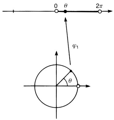
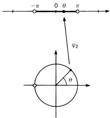
Let $m=1$ and require that $M$ be connected. There are only two manifolds possible: a real line $\mathbb{R}$ and the circle $S^1$ . Let us work out an atlas of $S^1$ . For concreteness take the circle $x^2+y^1=1$ in the $xy$ -plane. We need at least two charts. We may take them as in figure 5.4. Define ${\phi }_1^{-1}:(0,2\pi )\to S^1$ by

Figure 5.4. Two charts of a circle $S^1$ .

$${\phi }_1^{-1}:\theta \mapsto (\cos \theta ,\sin \theta )\text{\hspace{1em}(5.5a)}$$

whose image is $S^1-\{(1,0)\}$ . Define also ${\psi }_2^{-1}:(-\pi ,\pi )\to S^1$ by

$${\phi }_2^{-1}:\theta \mapsto (\cos \theta ,\sin \theta )\text{\hspace{1em}(5.5b)}$$

whose image is $S^1-\{(-1,0)\}$ . Clearly ${\phi }_1^{-1}$ and ${\phi }_2^{-1}$ are invertible and all the maps ${\phi }_1,{\phi }_2,{\phi }_1^{-1}$ and ${\phi }_2^{-1}$ are continuous. Thus, ${\phi }_1$ and ${\phi }_2$ are homeomorphisms. Verify that the maps ${\psi }_{12}={\phi }_1\circ {\phi }_2^{-1}$ and ${\psi }_{21}={\phi }_2\circ {\phi }_1^{-1}$ are smooth.

Example 5.3

The $n$ -dimensional sphere $S^n$ is a differentiable manifold. It is realized in ${\mathbb{R}}^{n+1}$ as

$$\sum _{i=0}^n{\left(x^i\right)}^2=1.\text{\hspace{1em}(5.6)}$$

Let us introduce the coordinate neighbourhoods

$$U_{i+}\equiv \left\{\left(x^0,x^1,\dots ,x^n\right)\in S^n\mid x^i>0\right\}\text{\hspace{1em}(5.7a)}$$

$$U_{i-}\equiv \left\{\left(x^0,x^1,\dots ,x^n\right)\in S^n\mid x^i<0\right\}.\text{\hspace{1em}(5.7b)}$$

Define the coordinate map ${\phi }_{i+}:U_{i+}\to {\mathbb{R}}^n$ by

$${\phi }_{i+}\left(x^0,\dots ,x^n\right)=\left(x^0,\dots ,x^{i-1},x^{i+1},\dots ,x^n\right)\text{\hspace{1em}(5.8a)}$$

and ${\phi }_{i-}:U_{i-}\to {\mathbb{R}}^n$ by

$${\phi }_{i-}\left(x^0,\dots ,x^n\right)=\left(x^0,\dots ,x^{i-1},x^{i+1},\dots ,x^n\right).\text{\hspace{1em}(5.8b)}$$

Note that the domains of ${\phi }_{i+}$ and ${\phi }_{i-}$ are different. ${\phi }_{i\pm }$ are the projections of the hemispheres $U_{i\pm }$ to the plane $x^i=0$ . The transition functions are easily obtained from (5.8). Take $S^2$ as an example. The coordinate neighbourhoods are $U_{x\pm },U_{y\pm }$ and $U_{z\pm }$ . The transition function ${\psi }_{y-x+}\equiv {\phi }_{y-}\circ {\phi }_{x+}^{-1}$ is given by

$${\psi }_{y-x+}:(y,z)\mapsto \left(\sqrt{1-y^2-z^2},z\right)\text{\hspace{1em}(5.9)}$$

which is infinitely differentiable on $U_{x+}\cap U_{y-}$ .

Exercise 5.1

At the beginning of this chapter, we introduced the stereographic coordinates on $S^2$ . We may equally define the stereographic coordinates projected from points other than the North Pole. For example, the stereographic coordinates $(U,V)$ of a point in $S^2-\{\text{South Pole}\}$ projected from the South Pole and $(X,Y)$ for a point in $S^2-\{\text{North Pole}\}$ projected from the North Pole are shown in figure 5.5. Show that the transition functions between $(U,V)$ and $(X,Y)$ are $C^{\infty }$ and that they define a differentiable structure on $M$ . See also example 8.1.

Figure 5.5. Two stereographic coordinate systems on $S^2$ . The point $P$ may be projected from the North Pole N giving $(X,Y)$ or from the South Pole S giving $(U,V)$ .

Example 5.4

The real projective space $\mathbb{R}{P}^n$ is the set of lines through the origin in ${\mathbb{R}}^{n+1}$ . If $x=(x^0,\dots ,x^n)\ne 0$ , $x$ defines a line through the origin. Note that $y\in {\mathbb{R}}^{n+1}$ defines the same line as $x$ if there exists a real number $a\ne 0$ such that $y=ax$ . Introduce an equivalence relation $\sim$ by $x\sim y$ if there

exists $a\in \mathbb{R}-\{0\}$ such that $y=ax$ . Then $\mathbb{R}{P}^n=({\mathbb{R}}^{n+1}-\{0\})/\sim$ . The $n+1$ numbers $x^0,x^1,\dots ,x^n$ are called the homogeneous coordinates. The homogeneous coordinates cannot be a good coordinate system, since $\mathbb{R}{P}^n$ is an $n$ -dimensional manifold (an $(n+1)$ -dimensional space with a one-dimensional degree of freedom killed). The charts are defined as follows. First we take the coordinate neighbourhood $U_i$ as the set of lines with $x^i\ne 0$ , and then introduce the inhomogeneous coordinates on $U_i$ by

$${\xi }_{(i)}^j=x^j/x^i.\text{\hspace{1em}(5.10)}$$

The inhomogeneous coordinates

$${\xi }_{(i)}=({\xi }_{(i)}^0,{\xi }_{(i)}^1,\dots ,{\xi }_{(i)}^{i-1},{\xi }_{(i)}^{i+1},\dots ,{\xi }_{(i)}^n)$$

with ${\xi }_{(i)}^i=1$ omitted, are well defined on $U_i$ since $x^i\ne 0$ , and furthermore they are independent of the choice of the representative of the equivalence class since $x^j/x^i=y^j/y^i$ if $y=ax$ . The inhomogeneous coordinate ${\xi }_{(i)}$ gives the coordinate map ${\phi }_i:U_i\to {\mathbb{R}}^n$ , that is

$${\phi }_i:\left(x^0,\dots ,x^n\right)\mapsto \left(x^0/x^i,\dots ,x^{i-1}/x^i,x^{i+1}/x^i,\dots ,x^n/x^i\right)$$

where $x^i/x^i=1$ is omitted. For $x=(x^0,x^1,\dots ,x^n)\in U_i\cap U_j$ we assign two inhomogeneous coordinates, ${\xi }_{(i)}^k=x^k/x^i$ and ${\xi }_{(j)}^k=x^k/x^j$ . The coordinate

transformation ${\psi }_{ij}={\phi }_i\circ {\phi }_j^{-1}$ is

$${\psi }_{ij}:{\xi }_{(j)}^k\mapsto {\xi }_{(i)}^k=\left(x^j/x^i\right){\xi }_{(j)}^k.\text{\hspace{1em}(5.11)}$$

This is a multiplication by $x^j/x^i$ .

In example 4.12, we defined $\mathbb{R}{P}^n$ as the sphere $S^n$ with antipodal points identified. This picture is in conformity with the definition here. As a representative of the equivalence class $[x]$ , we may take points $|x|=1$ on a line through the origin. These are points on the unit sphere. Since there are two points on the intersection of a line with $S^n$ we have to take one of them consistently, that is nearby lines are represented by nearby points in $S^n$ . This amounts to taking the hemisphere. Note, however, that the antipodal points on the boundary (the equator of $S^n$ ) are identified by definition, $(x^0,\dots ,x^n)\sim -(x^0,\dots ,x^n)$ . This ‘hemisphere’ is homeomorphic to the ball $D^n$ with antipodal points on the boundary $S^{n-1}$ identified.

Example 5.5

A straightforward generalization of $\mathbb{R}{P}^n$ is the Grassmann manifold. An element of $\mathbb{R}{P}^n$ is a one-dimensional subspace in ${\mathbb{R}}^{n+1}$ . The Grassmann manifold $G_{k,n}(\mathbb{R})$ is the set of $k$ -dimensional planes in ${\mathbb{R}}^n$ . Note that $G_{1,n+1}(\mathbb{R})$ is nothing but $\mathbb{R}{P}^n$ . The manifold structure of $G_{k,n}(\mathbb{R})$ is defined in a manner similar to that of $\mathbb{R}{P}^n$ .

Let $M_{k,n}(\mathbb{R})$ be the set of $k\times n$ matrices of rank $k$ ( $k\le n$ ). Take $A=(a_{ij})\in M_{k,n}(\mathbb{R})$ and define $k$ vectors $a_i$ ( $1\le i\le k$ ) in ${\mathbb{R}}^n$ by $a_i=(a_{ij})$ . Since $\text{rank }A=k$ , $k$ vectors $a_i$ are linearly independent and span a $k$ -dimensional plane in ${\mathbb{R}}^n$ . Note, however, that there are infinitely many matrices in $M_{k,n}(\mathbb{R})$ that yield the same $k$ -plane. Take $g\in \mathrm{GL}(k,\mathbb{R})$ and consider a matrix $\bar{A}=gA\in M_{k,n}(\mathbb{R})$ . $\bar{A}$ defines the same $k$ -plane as $A$ , since $g$ simply rotates the basis within the $k$ -plane. Introduce an equivalence relation $\sim$ by $\bar{A}\sim A$ if there exists $g\in \mathrm{GL}(k,\mathbb{R})$ such that $\bar{A}=gA$ . We identify $G_{k,n}(\mathbb{R})$ with the coset space $M_{k,n}(\mathbb{R})/\mathrm{GL}(k,\mathbb{R})$ .

Let us find the charts of $G_{k,n}(\mathbb{R})$ . Take $A\in M_{k,n}(\mathbb{R})$ and let $\{A_1,\dots ,A_l\}$ , $l=\left(\genfrac{}{}{0ex}{}{n}{k}\right)$ , be the collection of all $k\times k$ minors of $A$ . Since $\text{rank }A=k$ , there exists some $A_{\alpha }$ ( $1\le \alpha \le l$ ) such that $\det A\ne 0$ . For example, let us assume the minor $A_1$ made of the first $k$ columns has non-vanishing determinant,

$$A=\left(A_1,\widetilde{A_1}\right)\text{\hspace{1em}(5.12)}$$

where $\widetilde{A_1}$ is a $k\times (n-k)$ matrix. Let us take the representative of the class to which $A$ belongs to be

$$A_1^{-1}\cdot A=\left(I_k,A_1^{-1}\cdot \widetilde{A_1}\right)\text{\hspace{1em}(5.13)}$$

where $I_k$ is the $k\times k$ unit matrix. Note that $A_1^{-1}$ always exists since $\det A_1\ne 0$ . Thus, the real degrees of freedom are given by the entries of the $k\times (n-k)$ matrix $A_1^{-1}\cdot {\tilde{A}}_1$ . We denote this subset of $G_{k,n}(\mathbb{R})$ by $U_1$ . $U_1$ is a coordinate neighbourhood whose coordinates are given by $k(n-k)$ entries of $A_1^{-1}\cdot {\tilde{A}}_1$ . Since $U_1$ is homeomorphic to ${\mathbb{R}}^{k(n-k)}$ we find that

$$\dim G_{k,n}(\mathbb{R})=k(n-k).\text{\hspace{1em}(5.14)}$$

In the case where $\det A_{\alpha }\ne 0$ , where $A_{\alpha }$ is composed of the columns $(i_1,i_2,\dots ,i_k)$ , we multiply $A_{\alpha }^{-1}$ to obtain the representative

$$\begin{array}{rl}& \text{c o l u m n}\to i_1{i}_2\dots i_k\\ & A_{\alpha }^{-1}\cdot A=\left(\begin{array}{ccccccc}\dots & 1& \dots & 0& \dots \dots & 0& \dots \\ \dots & 0& \dots & 1& \dots \dots & 0& \dots \\ \dots & \cdot & \dots & \cdot & \dots \dots & \cdot & \dots \\ \dots & 0& \dots & 0& \dots \dots & 1& \dots \end{array}\right)\end{array}\text{\hspace{1em}(5.15)}$$

where the entries not written explicitly form a $k\times (n-k)$ matrix. We denote this subset of $M_{k,n}(\mathbb{R})$ with $\det A_{\alpha }\ne 0$ by $U_{\alpha }$ . The entries of the $k\times (n-k)$ matrix are the coordinates of $U_{\alpha }$ .

The relation between the projective space and the Grassmann manifold is evident. An element of $M_{1,n+1}(\mathbb{R})$ is a vector $A=(x^0,x^1,\dots ,x^n)$ . Since the $\alpha$ th minor $A_{\alpha }$ of $A$ is a number $x^{\alpha }$ , the condition $\det A_{\alpha }\ne 0$ becomes $x^{\alpha }\ne 0$ . The representative (5.15) is just the inhomogeneous coordinate

$$\begin{array}{rl}& (x^{\alpha }{)}^{-1}\left(x^0,x^1,\dots ,x^{\alpha },\dots ,x^n\right)\\ & =\left(x^0/x^{\alpha },x^1/x^{\alpha },\dots ,x^{\alpha }/x^{\alpha }=1,\dots ,x^n/x^{\alpha }\right).\end{array}$$

Let $M$ be an $m$ -dimensional manifold with an atlas $\{(U_i,{\phi }_i)\}$ and $N$ be an $n$ -dimensional manifold with $\{(V_j,{\psi }_j)\}$ . A product manifold $M\times N$ is an $(m+n)$ -dimensional manifold whose atlas is $\{(U_i\times V_j),({\phi }_i,{\psi }_j)\}$ . A point in $M\times N$ is written as $(p,q)$ , $p\in M$ , $q\in N$ , and the coordinate function $({\phi }_i,{\psi }_j)$ acts on $(p,q)$ to yield $({\phi }_i(p),{\psi }_j(p))\in {\mathbb{R}}^{m+n}$ . The reader should verify that a product manifold indeed satisfies the axioms of definition 5.1.

Example 5.6

The torus $T^2$ is a product manifold of two circles, $T^2=S^1\times S^1$ . If we denote the polar angle of each circle as ${\theta }_i\mathrm{mod}2\pi$ ( $i=1,2$ ), the coordinates of $T^2$ are $({\theta }_1,{\theta }_2)$ . Since each $S^1$ is embedded in ${\mathbb{R}}^2$ , $T^2$ may be embedded in ${\mathbb{R}}^4$ . We often imagine $T^2$ as the surface of a doughnut in ${\mathbb{R}}^3$ , in which case, however, we inevitably have to introduce bending of the surface. This is an extrinsic feature brought about by the ‘embedding’. When we say ‘a torus is a flat manifold’, we refer to the flat surface embedded in ${\mathbb{R}}^4$ . See definition 5.3 for further details.

We may also consider a direct product of $n$ circles,

$$T^n=\underset{n}{\underbrace{S^1\times S^1\times \cdots \times S^1}}.$$

Clearly $T^n$ is an $n$ -dimensional manifold with the coordinates $({\theta }_1,{\theta }_2,\dots ,{\theta }_n)\mathrm{mod}2\pi$ . This may be regarded as an $n$ -cube whose opposite faces are identified, see figure 2.4 for $n=2$ .

Endnotes

Unplaced source note

Strictly speaking the distance between two longitudes in the northern part of the city is slightly

来源与版本

正文：英文 · OCR 机器稿 · 待校对

核对状态：OCR 机器稿 · 待校对

原书 PDF

来源版本：second-edition-local

来源 PDF SHA-256：fcd24c3371d092a8c699ccf5cf0765462924b6c48412804231076e8084b1940d

OCR 来源 SHA-256：0b6324f01172a3548cd34382e82fd8bfae574602b6b2cfaa357ba96bc2c35478

OCR 产物 SHA-256：4715765ce9187d2e05ceffd1ba60393d8ca0a21516189959038b000f17753da0