6.1 The Schwarzschild Solution

We have already met the simplest black hole solution back in Section 1.3: this is the Schwarzschild solution, with metric

$$d{s}^2=-\left(1-\frac{2GM}{r}\right)d{t}^2+{\left(1-\frac{2GM}{r}\right)}^{-1}d{r}^2+r^2(d{\theta }^2+{\sin }^2\theta d{\varphi }^2)\text{\hspace{1em}(6.1)}$$

It is not hard to show that this solves the vacuum Einstein equations $R_{\mu \nu }=0$ . Indeed, the calculations can be found in Section 4.2 where we first met de Sitter space. The Schwarzschild solution is a special case of the more general metric (4.9) with $f(r{)}^2=$ $1-2GM/r$ and it’s simple to check that this obeys the Einstein equation which, as we’ve seen, reduces to the simple differential equations (4.10) and (4.11).

M is for Mass

The Schwarzschild solution depends on a single parameter, M, which should be thought of as the mass of the black hole. This interpretation already follows from the relation to Newtonian gravity that we first discussed way back in Section 1.2 where we anticipated that the $g_{00}$ component of the metric should be (1.26)

$$g_{00}=-(1+2\Phi )$$

with Φ the Newtonian potential. We made this intuition more precise in Section 5.1.2 where we discussed the Newtonian limit. For the Schwarzschild metric, we clearly have

$$\Phi =-\frac{GM}{r}$$

which is indeed the Newtonian potential for a point mass M at the origin.

The black hole also provides an opportunity to roadtest the technology of Komar integrals developed in Section 4.3.3. The Schwarzschild spacetime admits a timelike Killing vector $K={\partial }_t$ . The dual one-form is then

$$K=g_{00}dt=-\left(1-\frac{2GM}{r}\right)dt$$

Following the steps described in Section 4.3.3, we can then construct the 2-form

$$F=dK=-\frac{2GM}{r^2}dr\wedge dt$$

which takes a form similar to that of an electric field, with the characteristic $1/r^2$ fall-of. The Komar integral instructs us to compute the mass by integrating

$$M_{\mathrm{Komar}}=-\frac{1}{8\pi G}{\int }_{{\mathbf{S}}^2}\star F$$

where ${\mathbf{S}}^2$ is any sphere with radius larger than the horizon $r=2GM$ . It doesn’t matter which radius we choose; they all give the same answer, just like all Gaussian surfaces outside a charge distribution give the same answer in electromagnetism. Since the area of a sphere at radius r is $4\pi r^2.$ the integral gives

$$M_{\mathrm{Komar}}=M$$

for the Schwarzschild black hole.

There’s something a little strange about the Komar mass integral. As we saw in Section 4.3.3, the 2-form $F=dK$ obeys something very similar to the Maxwell equations, $d\star F=0$ . But these are the vacuum Maxwell equations in the absence of any current, so we would expect any “electric charge” to vanish. Yet this “electric charge” is precisely the mass $M_{\mathrm{Komar}}$ which, as we have seen, is distinctly not zero. What’s happening is that, for the black hole, the mass is all localised at the origin $r=0$ , where the field strength F diverges.

We might expect that the Schwarzschild solution only describes something physically sensible when $M\ge 0$ . (The $M=0$ Schwarzschild solution is simply Minkowski spacetime.) However, the metric (6.1) is a solution of the Einstein equations for all values of M. As we proceed, we’ll see that the $M<0$ solution does indeed have some rather screwy features that make it unphysical.

6.1.1 Birkhoff’s Theorem

The Schwarzschild solution (6.1) is, it turns out, the unique spherically symmetric, asymptotically flat solution to the vacuum Einstein equations. This is known as the Birkhoff theorem. In particular, this means that the Schwarzschild solution does not just describe a black hole, but it describes the spacetime outside any non-rotating, spherically symmetric object, like a star.

Here we provide a sketch of the proof. The first half of the proof involves setting up a useful set of coordinates. First, we make use of the statement that the metric is spherically symmetric, which means that it has an $SO(3)$ isometry. One of the more fiddly parts of the proof is to show that any metric with such an isometry can be written in coordinates that make this isometry manifest,

$$d{s}^2=g_{\tau \tau }(\tau ,\rho )d{\tau }^2+2g_{\tau \rho }(\tau ,\rho )d\tau d\rho +g_{\rho \rho }(\tau ,\rho )d{\rho }^2+r^2(\tau ,\rho )d{\Omega }_2^2$$

Here $\tau$ and $\rho$ are some coordinates and $d{\Omega }_2^2$ is the familiar metric on ${\mathbf{S}}^2$

$$d{\Omega }_2^2=d{\theta }^2+{\sin }^2\theta d{\varphi }^2$$

The $SO(3)$ isometry then acts on this ${\mathbf{S}}^2$ in the usual way, leaving $\tau$ and $\rho$ untouched. This is said to be a foliation of the space by the spheres ${\mathbf{S}}^2$

The size of the sphere is determined by the function $r(\tau ,\rho )$ in the above metric. The next step in the proof is to change coordinates so that we work with $\tau$ and $r,$ rather than $\tau$ and $\rho .$ We’re then left with the metric

$$d{s}^2=g_{\tau \tau }(\tau ,r)d{\tau }^2+2g_{\tau r}(\tau ,r)d\tau dr+g_{rr}(\tau ,r)d{r}^2+r^{2}d{\Omega }_2^2$$

In fact there’s a subtlety in the argument above: for some functions $r(\tau ,\rho )$ , it’s not possible to exchange $\rho$ for $r.$ Examples of such functions include $r=$ constant and $r=\tau$ . We can rule out such counter-examples by insisting that asymptotically the spacetime looks like Minkowski space.

Our next step is to introduce a new coordinate that gets rid of the cross-term $g_{\tau r}.$ To this end, consider the a coordinate $\tilde{t}(\tau ,r)$ . Then

$$d{\tilde{t}}^2={\left(\frac{\partial \tilde{t}}{\partial \tau }\right)}^{2}d{\tau }^2+2\frac{\partial \tilde{t}}{\partial \tau }\frac{\partial \tilde{t}}{\partial r}d\tau dr+{\left(\frac{\partial \tilde{t}}{\partial r}\right)}^{2}d{r}^2$$

We can always pick a choice of $\tilde{t}(\tau ,r)$ so that the cross-term $g_{\tau r}$ vanishes in the new coordinates. We’re then left with the simpler looking metric,

$$d{s}^2=-f(\tilde{t},r)d{\tilde{t}}^2+g(\tilde{t},r)d{r}^2+r^{2}d{\Omega }_2^2$$

Where we’ve now included the expected minus sign in the temporal part of the metric, reflecting our chosen signature. This is as far as we can go making useful coordinate choices. To proceed, we need to use the Einstein equations. As always, this involves sitting down and doing a fiddly calculation. Here we present only the (somewhat surprising) conclusion: the vacuum Einstein equations require that

$$f(r,\tilde{t})=f(r)h(\tilde{t})\mathrm{and}g(r,\tilde{t})=g(r)$$

In other words, the metric takes the form

$$d{s}^2=-f(r)h(\tilde{t})d{\tilde{t}}^2+g(r)d{r}^2+r^{2}d{\Omega }_2^2$$

But we can always absorb that $h(\tilde{t})$ factor by redefining the time coordinate, so that $h(\tilde{t})d{\tilde{t}}^2=d{t}^2$ . Finally, we’re left with the a metric of the form

$$d{s}^2=-f(r)d{t}^2+g(r)d{r}^2+r^{2}d{\Omega }_2^2\text{\hspace{1em}(6.2)}$$

This is important. We assumed that the metric was spherically symmetric, but made no such assumption about the lack of time dependence. Yet the Einstein equations have forced this upon us, and the final metric (6.2) has two sets of Killing vectors. The first arises from the SO(3) isometry that we originally assumed, but the second is the timelike Killing vector $K={\partial }_t$ that has emerged from the calculation.

At this point we need to finish solving the Einstein equations. It turns out that they require $f(r)=g(r{)}^{-1}$ , so the metric (6.2) reduces to the simple ansatz (4.9) that we considered previously. The Schwarzschild solution (6.1) is the most general solution to the Einstein equations with vanishing cosmological constant.

The fact that we assumed only spherical symmetry, and not time independence, means that the Schwarzschild solution not only describes the spacetime outside a timeindependent star, but also outside a collapsing star, providing that the collapse is spherically symmetric.

A Closer Look at Time Independence

There are actually two, different meanings to “time independence” in general relativity.

A spacetime is said to be stationary if it admits an everywhere timelike Kililng vector field K. In asymptotically flat spacetimes, we usually normalise this so that $K^2\to -1$ asymptotically.

A spacetime is said to be static if it is stationary and, in addition, is invariant under $t\to -t.$ , where t is a coordinate along the integral curves of K. In particular, this rules out dt dX cross-terms in the metric, with X some other coordinate.

Birkhoff’s theorem tells us that spherical symmetry implies that the spacetime is necessarily static. In Section 6.3, we’ll come across spacetimes that are stationary but not static.

6.1.2 A First Look at the Horizon

There are two values of r where the Schwarzschild metric goes bad: $r=0$ and $r=2GM$ At each of these values, one of the components of the metric diverges but, as we will see, the interpretation of this divergence is rather different in the two cases. We will learn that the divergence at the point $r=0$ is because the spacetime is sick: this point is called the singularity. The theory of general relativity breaks down as we get close to the singularity and to make sense of what’s happening there we need to turn to a quantum theory of spacetime.

In contrast, nothing so dramatic happens at the surface $r=2GM$ and the divergence in the metric is merely because we’ve made a poor choice of coordinates: this surface is referred to as the event horizon, usually called simply the horizon. Many of the surprising properties of black holes lie in interpreting the event horizon.

There is a simple diagnostic to determine whether a divergence in the metric is due to a true singularity of the spacetime, or to a poor choice of coordinates. We build a scalar quantity that does not depend on the choice of coordinates. If this too diverges then it’s telling us that the spacetime itself is indeed sick at that point. If it does not diverge, we can’t necessarily conclude that the spacetime isn’t sick because there may be some other scalar quantity that signifies there is a problem. Nonetheless, we might start to wonder if perhaps nothing very bad happens.

The simplest scalar is, of course, the Ricci scalar. But this is necessarily $R=0$ for any vacuum solution to the Einstein equation so it is not helpful in detecting the nature of singularities. The same is true for $R_{\mu \nu }{R}^{\mu \nu }$ . For this reason, the simplest curvature diagnostic is the Kretschmann scalar, $R^{\mu \nu \rho \sigma }{R}_{\mu \nu \rho \sigma }$ . For the Schwarzschild solution it is given by

$$R^{\mu \nu \rho \sigma }{R}_{\mu \nu \rho \sigma }=\frac{48G^2{M}^2}{r^6}\text{\hspace{1em}(6.3)}$$

We see that the Kretschmann scalar exhibits no pathology at the surface $r=2GM$ 2 where $R^{\mu \nu \rho \sigma }{R}_{\mu \nu \rho \sigma }\sim 1/(GM{)}^4$ . This suggests that perhaps this divergence in the metric isn’t as worrisome as it may have first appeared. Note, moreover, that, perhaps counter-intuitively, heavier black holes have smaller curvature at the horizon. We see that this arises because such black holes are bigger and the $1/r^6$ factor beats the $M^2$ factor.

In contrast, the curvature indeed diverges at the origin $r=0$ , telling us that the spacetime is problematic at this point. Of course, given that we have still to understand the horizon at $r=2GM$ , it’s not entirely clear that we can trust the Schwarzschild metric for values $r<2GM$ . As we will proceed, we will see that the singularity at $r=0$ is a genuine feature of the (classical) black hole.

The Near Horizon Limit: Rindler Space

To understand what’s happening near the horizon $r=2GM$ , we can zoom in and look at the metric in the vicinity of the horizon. To do this, we write

$$r=2GM+\eta$$

where we take $\eta \ll 2GM$ . We further take $\eta >0$ which means that we’re looking at the region of spacetime just outside the horizon. We then approximate the components of the metric as

$$1-\frac{2GM}{r}\approx \frac{\eta }{2GM}\mathrm{and}{r}^2=(2GM+\eta {)}^2\approx (2GM{)}^2$$

To this order, the Schwarzschild metric becomes

$$d{s}^2=-\frac{\eta }{2GM}d{t}^2+\frac{2GM}{\eta }d{\eta }^2+(2GM{)}^{2}d{\Omega }_2^2$$

The first thing that we see is that the metric has decomposed into a direct product of an ${\mathbf{S}}^2$ of radius 2GM, and a $d=1+1$ dimensional Lorentzian geometry. We’ll focus on this 2d Lorentzian geometry. We make the change of variables

$${\rho }^2=8GM\eta$$

after which the 2d metric becomes

$$d{s}^2=-{\left(\frac{\rho }{4GM}\right)}^{2}d{t}^2+d{\rho }^2$$

This rather simple metric is known as Rindler space. It is, in fact, just Minkowski space in disguise. The disguise is the transformation

$$T=\rho \sinh \left(\frac{t}{4GM}\right)\text{ and }X=\rho \cosh \left(\frac{t}{4GM}\right)\text{\hspace{1em}(6.4)}$$

after which the metric becomes

$$d{s}^2=-d{T}^2+d{X}^2\text{\hspace{1em}(6.5)}$$

We’ve met something very similar to the coordinates (6.4) previously: they are the coordinates experienced by an observer undergoing constant acceleration $a=1/4GM$ where t is the proper time of this observer. (We saw such coordinates earlier in (1.25) which differ only by a constant offset to the spatial variable $\rho .)$ This makes sense: an observer who sits at a constant $\rho$ value, corresponding to a constant r value, must accelerate in order to avoid falling into the black hole.

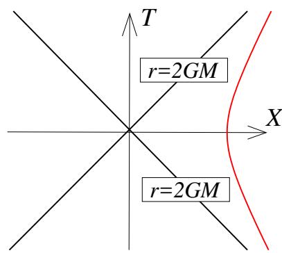
Figure 31. The near horizon limit of a black hole is Rindler spacetime, with the null lines $X=\pm T$ corresponding to the horizon at $r=2GM$ . Also shown in red is a line of constant $r>2GM$ outside the black hole.

We can now start to map out what part of Minkowski space (6.5) corresponds to the outside of the black hole horizon. This is $\rho >0$ and $t\in (-\infty ,+\infty )$ . From the change of variables (6.4), we see that this corresponds the region $X>|T|$

We can also see what becomes of the horizon itself. This sits at $r=2GM$ , or $\rho =0$ For any finite t, the horizon $\rho =0$ gets mapped to the origin of Minkowski space, $X=T=0$ . However, the time coordinate is degenerate at the horizon since $g_{00}=0$ If we scale $t\to \infty$ , and $\rho \to 0$ keeping the combination $\rho e^{\pm t/4GM}$ fixed, then we see that the horizon actually corresponds to the lines:

$$r=2GM\Rightarrow X=\pm T$$

This is our first lesson. The event horizon of a black hole is not a timelike surface, like the surface of a star. Instead it is a null surface. This is depicted in Figure 31.

Although our starting point was restricted to coordinates X and T given by (6.4), once we get to the Minkowski space metric (6.5) there’s no reason to retain this restriction. Indeed, clearly the metric makes perfect sense if we extend the range of the coordinates to $X,T\in \mathbf{R}$ . Moreover, this metric makes it clear that nothing fishy is happening at the horizon $X=\pm |T|$ . We see that if we zoom in on the horizon, then it’s no different from any other part of spacetime. Nonetheless, as we go on we will learn that the horizon does have some rather special properties, but you only get to see them if you look at things from a more global perspective.

6.1.3 Eddington-Finkelstein Coordinates

Above we saw that, in the near-horizon limit, a clever change of variables allows us to remove the coordinate singularity at the horizon and extend the spacetime beyond. Our goal in this section is to play the same game, but now for the full black hole metric.

Before we proceed, it’s worth commenting on the logic here. When we first met differential geometry in Section 2, we made a big deal of the fact that a single set of coordinates need not cover the entire manifold. Instead, one typically needs different coordinates in different patches, together with transition functions that relate the coordinates where the patches overlap. The situation with the black hole is similar, but not quite the same. It’s true that the coordinates of the Schwarzschild metric (6.1) do not cover the entire spacetime: they break down at $r=2GM$ and it’s not clear that we should trust the metric for $r<2GM$ . But rather than finding a new set of coordinates in the region beyond the horizon, and trying to patch this together with our old coordinates, we’re instead going to find a new set of coordinates that works everywhere.

Our first step is to introduce a new radial coordinate, $r_{\star },$ defined by

$$d{r}_{\star }^2={\left(1-\frac{2GM}{r}\right)}^{-2}d{r}^2\text{\hspace{1em}(6.6)}$$

The solution to this differential equation is straightforward to find: it is

$$r_{\star }=r+2GM\log \left(\frac{r-2GM}{2GM}\right)\text{\hspace{1em}(6.7)}$$

We see that the region outside the horizon $2GM<r<\infty$ maps to $-\infty <r_{\star }<+\infty$ in the new coordinate. As we approach the horizon, the change in r is increasingly slow as we vary $r_{\star }$ (since $dr/d{r}_{\star }\to 0\mathrm{as}r\to 2GM.)$ For this reason it is called the tortoise coordinate. (It is also sometimes called the Regge-Wheeler radial coordinate.)

The tortoise coordinate is well adapted to describe the path of light rays travelling in the radial direction. Such light rays follow curves satisfying

$$d{s}^2=0\Rightarrow \frac{dr}{dt}=\pm \left(1-\frac{2GM}{r}\right)\Rightarrow \frac{d{r}_{\star }}{dt}=\pm 1$$

We see that null, radial geodesics are given by

$$t\pm r_{\star }=\mathrm{constant}$$

where the plus sign corresponds to ingoing geodesics (as t increases, $r_{\star }$ must decrease) and the negative sign to outgoing geodesics.

Next, we introduce a pair of null coordinates

$$v=t+r_{\star }\mathrm{and}u=t-r_{\star }$$

In what follows we will consider the Schwarzschild metric written first in coordinates $(v,r)$ , then in coordinates $(u,r)$ and finally, in Section 6.1.4, in coordinates $(u,v)$

Ingoing Eddington-Finkelstein Coordinates

As a first attempt to extend the Schwarzschild solution beyond the horizon, we replace t with $t=v-r_{\star }(r)$ . We have

$$dt=dv-d{r}_{\star }=dv-{\left(1-\frac{2GM}{r}\right)}^{-1}dr$$

Making this substitution in the Schwarzschild metric (6.1), we find the new metric

$$d{s}^2=-\left(1-\frac{2GM}{r}\right)d{v}^2+2dvdr+r^{2}d{\Omega }_2^2\text{\hspace{1em}(6.8)}$$

This is the Schwarzschild black hole in ingoing Eddington-Finkelstein coordinates. We see that the $d{r}^2$ terms have now disappeared, and so there is no singularity in the metric at $r=2GM$ . However, the $d{v}^2$ term vanishes at $r=2GM$ and, moreover, flips sign for $r<2GM$ . You might worry that this means that the coordinates still go bad there, or even that the signature of the metric changes as we cross the horizon. To allay such worries, we need only compute the determinant of the metric

$$\det (g)=\det \left(\begin{array}{cccc}-(1-\frac{2GM}{r})& 1& 0& 0\\ 1& 0& 0& 0\\ 0& 0& r^2& 0\\ 0& 0& 0& r^2{\sin }^2\theta \end{array}\right)=-r^4{\sin }^2\theta$$

We see that the dv dr cross-term stops the metric becoming degenerate at the horizon and the signature remains Lorentzian for all values of r. (The metric is still degenerate at the $\theta =0,\pi$ but these are simply the poles of the ${\mathbf{S}}^2$ and we know how to deal with that.)

This, then, is the advantage of the ingoing Eddington-Finkelstein coordinates: the r coordinate can be continued past the horizon, all the way down to the singularity at $r=0$

The original Schwarzschild metric (6.1) was time independent. Mathematically, this follows from the statement that the metric exhibits a timelike Killing vector $K={\partial }_t$ This Killing vector also exists in the Eddington-Finkelstein extension, where it is now $K:=:{\partial }_v$ . The novelty is that this Killing vector is no longer everywhere timelike. Instead, it remains timelike outside the horizon where $g_{vv}<0$ , but becomes spacelike inside the horizon where $g_{vv}>0$ . In other words, the full black hole geometry is not time independent! We’ll learn more about this feature as we progress.

The Finkelstein Diagram

To build further intuition for the geometry, we can look at the behaviour of light rays coming out of the black hole. These follow paths given by

$$u=t-r_{\star }=\mathrm{constant}$$

Eliminating $t,$ in preference of the null coordinate $v=t+r_{\star }$ , outgoing null geodesics satisfy $v=2r_{\star }+\mathrm{constant}$ . The solutions to this equation have a different nature depending on whether we are outside or inside the horizon. For $r>2GM$ , we can use the original definition (6.7) of the tortoise coordinate $r_{\star }$ to get

$$v=2r+4GM\log \left(\frac{r-2GM}{2GM}\right)+\mathrm{constant}$$

Clearly the log term goes bad for $r<2GM$ . However, it is straightforward to write down a tortoise coordinate that obeys (6.6) on either side of the horizon: we simply need to take the modulus of the argument

$$r_{\star }=r+2GM\log \left|\frac{r-2GM}{2GM}\right|$$

This means that $r_{\star }$ is multi-valued: it sits in the range $r_{\star }\in (-\infty ,+\infty )$ outside the horizon, and in the range $r_{\star }\in (-\infty ,0)$ inside the horizon, with the singularity at $r_{\star }=0$ . Outgoing geodesics inside the horizon then obey

$$v=2r+4GM\log \left(\frac{2GM-r}{2GM}\right)+\mathrm{constant}\text{\hspace{1em}(6.9)}$$

It remains to find the outgoing null geodesic at the horizon $r=2GM$ . Here the $d{v}^2$ term in the metric (6.8) vanishes, and one can check that the surface $r=2GM$ is itself a null geodesic. This agrees with our expectation from Section 6.1.2 where we saw that the horizon is a null surface.

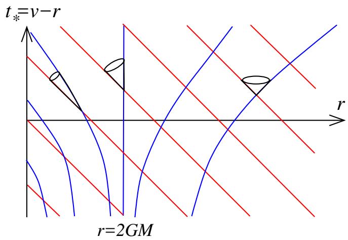
Figure 32. The Finkelstein diagram in ingoing coordinates. Ingoing null geodesics and shown in red, outgoing in blue. Inside the horizon at $r=2GM$ , outgoing geodesics do not go out.

We can capture this information in a Finkelstein diagram. This is designed so that ingoing null rays travel at 45 degrees. This is simple to do if we label the coordinates of the diagram by t and $r_{\star }$ . However, as we’ve seen, $r_{\star }$ isn’t single valued everywhere in the black hole. For this reason, we will label the spatial coordinate by the original r. We then define a new temporal coordinate $t_{\star }$ by the requirement

$$v=t+r_{\star }=t_{\star }+r$$

So ingoing null rays travel at 45 degrees in the $(t_{\star },r)$ plane, where $t_{\star }=v-r$ . These are shown as the red lines in Figure 32. Meanwhile, the outgoing null geodesics are shown in blue. Now we can clearly see how the behaviour changes depending on whether the geodesics are inside or outside the horizon. The outgoing geodesics that sit outside the horizon do what their name suggests: they move out. In particular, as $t\to \infty$ (so $t_{\star }\to \infty )$ , the geodesics escape to $r\to \infty$

The outgoing geodesics that sit inside the horizon are not so lucky. Now as t increases, the geodesics described by (6.9) don’t go “out” at all: instead the “outgoing” light rays move inexorably towards the curvature singularity at $r=0$ . Each of them hits the singularity at some finite $t_{\star }$

Bounding these two regions are the null geodesics which simply run along the horizon $r=2GM$ : this is the vertical blue line in the figure.

We can also draw light-cones on the Finkelstein diagram. These are the regions bounded by the ingoing and outgoing, future-pointing null geodesics, as shown in the figure. Any massive particle must follow a timelike path, and hence its trajectory must sit within these lightcones. We see immediately one of the key features of black holes: if you venture into past the horizon, you’re not getting back out again. This is forbidden by the causal structure of the spacetime. The term black hole really refers to the region $r<2GM$ inside the horizon. Any observer who remains outside the horizon can know nothing about what’s happening inside.

We can also use the Finkelstein diagram to tell us what an observer will see if they push their friend into a black hole. The hapless companion sails through the horizon, quite possibly without realising anything is wrong. However, any light signals that are sent back take longer and longer to reach an observer sitting at some fixed radial value $r>2GM$ . This means that the actions of the in-falling friend become increasingly slowed down as they approach the horizon. In this way, the observer/villain sitting outside continues to see their friend forever, but knows nothing of their action after they cross the horizon. Furthermore, since the light is now emerging from a deeper and deeper gravitational well, it will appear increasingly redshifted to the outside observer.

Outgoing Eddington-Finkelstein Coordinates

There is a different extension of the exterior of the Schwarzschild black hole, in which we replace the time coordinate t with the null coordinate

$$u=t-r_{\star }$$

Recall the surfaces of constant u correspond to outgoing, radial, null geodesics.

As before, it is straightforward to make this change of variable. We have $t=u+r_{\star }$ 2 so

$$dt=du+d{r}_{\star }=du+{\left(1-\frac{2GM}{r}\right)}^{-1}dr$$

Making this substitution in the Schwarzschild metric (6.1), we now find the metric

$$d{s}^2=-\left(1-\frac{2GM}{r}\right)d{u}^2-2dudr+r^{2}d{\Omega }_2^2\text{\hspace{1em}(6.10)}$$

This is the Schwarzschild solution in outgoing Eddington-Finkelstein coordinates. The only difference with the ingoing coordinates (6.8) is the sign of the cross-term. However, as we now explain, this seemingly trivial difference greatly changes the interpretation of the metric.

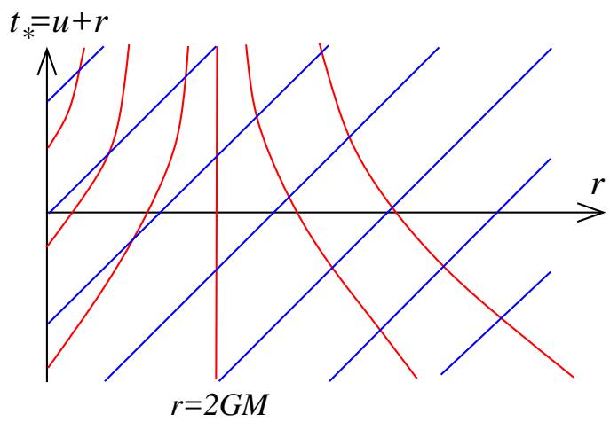
Figure 33. The Finkelstein diagram in outgoing coordinates. Ingoing null geodesics are shown in red, outgoing in blue. Inside the horizon at $r=2GM$ , ingoing geodesics do not go in.

Once again, the metric is smooth (and non-degenerate) at the horizon so we can happily continue the metric down to the singularity at $r=0$ . However, the region $r<2GM$ now describes a different part of spacetime from the analogous region in ingoing Eddington-Finkelstein coordinates!

To see this, we can again look at the ingoing and outgoing geodesics, as seen in the Finkelstein diagram in Figure 33. This time, we pick coordinates so that the outgoing geodesics travel at 45 degrees. This means that we take r and $t_{\star }=u+r$ . The outgoing geodesics are drawn in red as before. But this time we see that they do what their name suggests: they go always go out, regardless of whether they start life behind the horizon.

This time, it is the ingoing null geodesics that have the interesting property. Those that start life outside are unable to reach the singularity. Instead, they pile up at the horizon. Those that start life behind the horizon have an even stranger property: the ingoing geodesics do not go in. Instead they too move towards the horizon, again unable to cross it.

We can also ask what becomes of massive particles that sit inside the horizon. As before, their trajectories must lie within future-pointing light cones. We see that they cannot linger inside the horizon for long. The causal structure of the spacetime ultimately ejects them into the region outside the horizon.

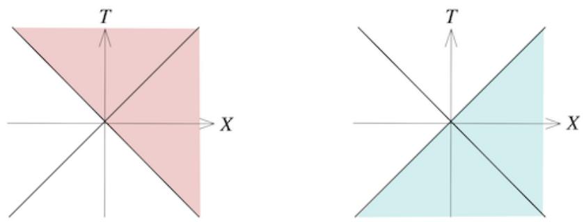
Figure 34. On the left: ingoing coordinates cover this part of Rindler space. On the right: outgoing coordinates cover this part.

This is clearly very different physics from a black hole. Instead, the solution (6.10) is that of a white hole, an object which expels any matter inside. This is the time reversal of a black hole, a fact which can be traced to the relative minus sign between the two metrics (6.8) and (6.10). This time reversal is also manifest in the diagrams: turn the white hole of Figure 33 upside down and you get the black hole of Figure 32.

White holes are perfectly acceptable solutions to the Einstein equations. Indeed, given the existence of black holes from which nothing can escape, the time reversal invariance of the Einstein equations tells us that there had to be a corresponding solution which nothing can enter. Nonetheless, white holes are not physically relevant since, in contrast to black holes, one cannot form them from collapsing matter.

6.1.4 Kruskal Spacetime

It may be somewhat surprising to learn that we can extend the $r\in (2GM,\infty )$ coordinate of the Schwarzschild solution in two different ways, so what we gain — the region parameterised by $r\in (0,2GM]$ — corresponds to two different parts of spacetime! We can gain some intuition for this by returning to the near horizon limit of Rindler space. The region outside the black hole, covered by the Schwarzschild metric, corresponds to the right-hand quadrant of Rindler space. The ingoing Eddington-Finkelstein coordinates extend this to the upper quadrant, while the outgoing Eddington-Finkelstein coordinates extend it to the lower quadrant, as shown in the figures above. The purpose of this section is to understand this better. We will achieve this by introducing coordinates which cover the entire spacetime, including both black and white holes.

It is simple to write the Schwarzschild metric using both null coordinates $v=t+r_{\star }$ and $u=t-r_{\star }$ . It becomes

$$d{s}^2=-\left(1-\frac{2GM}{r}\right)dudv+r^{2}d{\Omega }_2^2\text{\hspace{1em}(6.11)}$$

where we should now view $r^2$ as a function $r^2(u-v)$ . In these coordinates, the metric is degenerate at $r=2GM$ so we need to do somewhat better. This can be achieved by introducing the Kruskal-Szekeres coordinates,

$$U=-\exp \left(-\frac{u}{4GM}\right)\mathrm{and}V=\exp \left(\frac{v}{4GM}\right)\text{\hspace{1em}(6.12)}$$

Both U and V are null coordinates. As defined above, the exterior of the Schwarzschild black hole is parameterised by $U<0$ and $V>0$ . They have the further property that, outside the horizon,

$$UV=-\exp \left(\frac{r_{\star }}{2GM}\right)=\frac{2GM-r}{2GM}\exp \left(\frac{r}{2GM}\right)\text{\hspace{1em}(6.13)}$$

where, in the second equality, we’ve used the definition (6.7) of the tortoise coordinate. Similarly,

$$\frac{U}{V}=-\exp \left(-\frac{t}{2GM}\right)\text{\hspace{1em}(6.14)}$$

A quick calculation shows that the metric (6.11) becomes

$$d{s}^2=-\frac{32(GM{)}^3}{r}{e}^{-r/2GM}dUdV+r^{2}d{\Omega }_2^2\text{\hspace{1em}(6.15)}$$

where $r(U,V)$ is the function defined by inverting (6.13).

The original Schwarzschild metric covers only the region of spacetime with $U<0$ and $V>0$ . But now we can happily extend the range to $U,V\in \mathbf{R}$ , with the function $r(U,V)$ again defined by (6.13). We see that now nothing bad happens at $r=2GM$ the metric is smooth and non-degenerate.

Analytic Extensions

Given the amount of games we’ve played above, jumping between different coordinate systems, one may wonder if there are further games in which the Kruskal spacetime can be extended yet further. This turns out not to be the case: the Kruskal spacetime is the maximal extension of the Schwarzschild solution.

Here is the way to check whether a given spacetime can be extended: look at all geodesics and see where they end up. If you can follow geodesics for infinite affine parameter, then they escape to infinity. If, on the other hand, geodesics come to an end at some finite affine parameter then something is going on: either they run into a genuine singularity, or they run into a coordinate singularity. In the former case there’s nothing you can do about it. In the latter case, you can extend the spacetime as we have above. You have the maximally extended spacetime when any geodesics that come to an abrupt halt do so at genuine singularities.

There is something a little magical about the extension process. We start of with a solution to the Einstein equations in some region of spacetime. Yet this is sufficient to determine the metric throughout the entire, extended spacetime. In particular, once we’ve extended, we don’t have to solve the Einstein equations from scratch. This magic follows from the fact that the metric components are real, analytic functions. This means that knowledge of the metric in any open set is sufficient to determine it everywhere.

The Kruskal Diagram

We can see what becomes of the horizon in the new coordinates by using (6.13). We have

$$r=2GM\Rightarrow U=0\mathrm{or}V=0$$

This tells us that the horizon is not one null surface, but two null surfaces, intersecting at the point $U=V=0$ . This agrees with what we learned from taking the near horizon limit where we encountered Rindler space. The null surface U = 0 is the horizon of the black hole; it is called the future horizon. The null surface V = 0 is the horizon of the white hole; it is the past horizon.

We can also see what becomes of the singularity. This now sits at

$$r=0\Rightarrow UV=1$$

The hyperbola UV = 1 has two disconnected components. One of these, with $U,V>0$ corresponds to the singularity of the black hole. The other, with $U,V<0$ corresponds to the singularity of the white hole.

These facts can be depicted on a Kruskal diagram, shown in Figure 35. The U and V axes are drawn at 45 degrees, reflecting the fact that they are null lines. These are the two horizons. In this diagram, the vertical direction can be viewed as the time

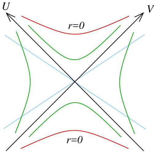
Figure 35. The Kruskal diagram for the Schwarzschild black hole. The U and V axes are the horizons at $r=2GM$ and the red lines are the singularities at $r=0$ . Also shown are lines of constant r in green, and lines of constant t in blue.

$T=\frac{1}{2}(V+U)$ while the horizontal spatial direction is $X=\frac{1}{2}(V-U)$ . The singularities $UV=1$ are drawn in red. This diagram makes it clear how the black hole and white hole cohabit in the same spacetime.

The diagram also shows lines of constant r, drawn in green, and lines of constant t drawn in blue. From (6.13), we see that lines of constant r are given by $UV=\mathrm{constant}$ Meanwhile, from (6.14), lines of constant t are linear, given by $U/V=\mathrm{constant}$

The diagram contains some important lessons. You might have naively thought that the singularity of the black hole was a point that traced a timelike worldline, similar to any other particle. The diagram makes it clear that this is not the case: instead, the singularity is spacelike. Once you pass through the horizon, the singularity isn’t something that sits to your left or to your right: it is something that lies in your future. This makes it clear why you cannot avoid the singularity when inside a black hole. It is your fate. Similarly, the singularity of the white hole lies in the past. It is similar to the singularity of the Big Bang.

We can frame this in terms of the Killing vector of the Schwarzschild solution $K={\partial }_t$ This is timelike outside the horizon and, indeed, gives rise to the conserved energy of geodesics outside the black hole that we met in Section 1.3. In the Kruskal coordinates,

we can use (6.12) to find

$$K=\frac{\partial }{\partial t}=\frac{\partial V}{\partial t}\frac{\partial }{\partial V}+\frac{\partial U}{\partial t}\frac{\partial }{\partial U}=\frac{1}{4GM}\left(V\frac{\partial }{\partial V}-U\frac{\partial }{\partial U}\right)$$

Evaluating the norm of this Killing vector in the Kruskal metric (6.15), we have

$$g_{\mu \nu }{K}^{\mu }{K}^{\nu }=-\left(1-\frac{2GM}{r}\right)$$

We see that outside the horizon, the Killing vector is timelike as expected. But inside the horizon, with $r<2GM$ , the Killing vector is spacelike. (We saw similar behaviour when discussing the isometries of de Sitter space in Section 4.3.1.) When we say that a spacetime is time independent, we mean that there exists a timelike Killing vector. We learn that the full black hole spacetime is not time independent. But this only becomes apparent once you cross the horizon.

A hint of this, albeit one that cannot be trusted, can be seen in the original Schwarzschild solution (6.1). If we were to take this at face value for $0<r<2GM$ , we see that the change of sign in $(1-2GM/r)$ means that the vector ${\partial }_t$ becomes spacelike and the vector ${\partial }_r$ timelike. This again suggests that the singularity lies in the future or the past. All the hard work in changing coordinates above shows that this naive result is, in fact, true.

The Einstein-Rosen Bridge

We now understand three of the four quadrants of the Kruskal diagram. The righthand quadrant is the exterior of the black hole, which is the spacetime covered by the original Schwarzschild coordinates. The upper quadrant is the interior of the black hole and the lower quadrant is the interior of the white hole. This leaves the left-hand quadrant. This is a surprise: it is another copy of the exterior of the black hole, now covered by $U>0$ and $V<0$ . To see this, we can write

$$U=+\exp \left(-\frac{u}{4GM}\right)\mathrm{and}V=-\exp \left(\frac{v}{4GM}\right)$$

Going back through the various coordinate transformations then shows that the lefthand quadrant is again described by the Schwarchild metric.

What are we to make of this? Our final spacetime contains two asymptotically flat regions joined together by a black hole! That sounds rather wild. Note that it’s not possible for an observer in one region to send a signal to an observer in another because the causal structure of the spacetime does not allow this. Nonetheless, we could ask: what is the spatial geometry that connects the two regions?

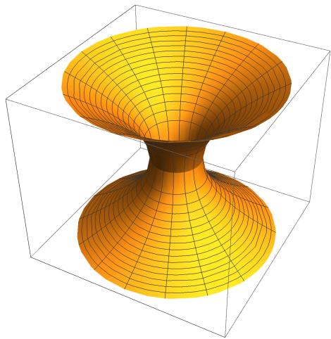
Figure 36. The Einstein-Rosen Bridge

To elucidate this spatial geometry, we look at the $t=0$ slice of Kruskal spacetime. This is $\mathrm{a}$ straight, horizontal line passing through $U=V=0$ . If we return to our original Schwarzschild metric then, at $t=0$ , the spatial geometry is given by

$$d{s}^2={\left(1-\frac{2GM}{r}\right)}^{-1}d{r}^2+r^2(d{\theta }^2+{\sin }^2\theta d{\varphi }^2)\text{\hspace{1em}(6.16)}$$

which is valid for $r>2GM$ . This describes the geometry in the right-hand quadrant. There is another copy of the same geometry in the left-hand quadrant. We then glue these together at $r=2GM$ , to give a wormhole-like geometry as shown in Figure 36. This wormhole is called the Einstein-Rosen bridge. It’s not a wormhole that you can travel through because the paths are spacelike, not timelike.

It’s possible to write down a metric that includes both sides of the wormhole. To do this we introduce a new radial coordinate $\rho ,$ defined by

$$r=\rho {\left(1+\frac{GM}{2\rho }\right)}^2=\rho +GM+\frac{G^2{M}^2}{4\rho }\text{\hspace{1em}(6.17)}$$

This is plotted in the figure. It has the property that there are two values of $\rho$ for each value of

$r>2GM$ . At the horizon, $r=2GM$ , there is just a single value: $\rho =GM/2$ . The idea is that $\rho >GM/2$ parameterises one side of the wormhole while $\rho <GM/2$ parameterises the other. Substituting $r$ for $\rho$ in (6.16) gives the metric

$$d{s}^2={\left(1+\frac{GM}{2\rho }\right)}^4\left[d{\rho }^2+{\rho }^2(d{\theta }^2+{\sin }^2\theta d{\varphi }^2)\right]\text{\hspace{1em}(6.18)}$$

(To show this, it’s useful to first show that $(1-2GM/r)=(1-GM/2\rho {)}^2(1+2GM/\rho {)}^{-2}.)$ Clearly this metric looks like flat ${\mathbf{R}}^3$ as $\rho \to \infty$ since we can drop the overall factor. Less obviously, it also looks like flat ${\mathbf{R}}^3$ as $\rho \to 0$ . To see this, note that there is a symmetry of (6.17) under $\rho \to G^2{M}^2/4\rho .$ , which swaps the two asymptotic spacetimes, leaving the meeting point at $\rho =GM/2$ invariant. In this way, the metric (6.18) describes the two-sided Einstein-Rosen bridge shown in Figure 36.

The radius of the ${\mathbf{S}}^2$ is 2GM in the middle of the wormhole at $\rho =GM/2$ , and then grows as we move away in either direction. This middle point is where the two horizons $U=0$ and $V=0$ meet. In fancy language, it is called the bifurcation sphere.

ER = EPR?

Although there is no way that an observer in the left-most quadrant can signal to an observer in the right-most quadrant, there is one way in which they can communicate: both need to be brave and jump into the black hole. Then they can both meet behind the horizons and share their stories.

This sounds like a rather wild idea! Is it physically meaningful? After all, the white hole that sits in the bottom quadrant is thought to have no physical manifestation. Similarly, it seems likely that for generic black holes the other universe that appeared in the left quadrant of the Kruskal diagram is also a mathematical artefact. Nonetheless, there is one rather speculative proposal in which such communication behind the horizon may be possible.

First, we can dispel the idea that the two asymptotic regimes necessarily correspond to different universes. One could patch together the asymptotic parts of the two Minkowski spaces so that the Kruskal diagram gives an approximate description of two, far separated black holes in the same universe. This would be an approximate solution to the field equations since, no matter how far, the two black holes would attract.

Viewed in this way, the Kruskal diagram suggests that two observers, potentially living billions of light years apart, could jump into these far flung black holes and meet behind the horizon. They could then have a nice chat before their inevitable demise in the singularity. Is this outlandish idea possible? And, if so, which pairs of black holes in the universe are connected in this way?

A proposal, emerging from ideas in quantum gravity, suggests that two black holes are connected in this way if they have some measure of quantum entanglement. This proposal goes by the cute name of $\mathrm{ER}=\mathrm{EPR}$ , with ER denoting the Einstein-Rosen bridge characterising a geometric connection, and EPR denoting the entanglement of the Einstein-Podolosky-Rosen paradox. (More details of entanglement can be found in the lectures on Topics in Quantum Mechanics.) It is far from clear that the $\mathrm{ER}=\mathrm{EPR}$ proposal is correct, but it is certainly a tantalising idea.

The Penrose Diagram

As we explained in Section 4.4.2, the best way to exhibit the causal structure of a spacetime is to draw the Penrose diagram. For the black hole, this is very similar to the Kruskal diagram: we simply straighten out a few lines.

The first step is to introduce new coordinates which cover the entire space in a finite range. We use the same kind of transformation that we saw in many examples in Section 4.4.2, namely

$$U=\tan \tilde{U}\mathrm{and}V=\tan \tilde{V}$$

The new coordinates have finite range $\tilde{U},\tilde{V}\in (-\pi /2,+\pi /2)$ . The Kruskal metric (6.15) is then

$$d{s}^2=\frac{1}{{\cos }^2\tilde{U}{\cos }^2\tilde{V}}\left[-\frac{32(GM{)}^3}{r}{e}^{-r/2GM}d\tilde{U}d\tilde{V}+r^2{\cos }^2\tilde{U}{\cos }^2\tilde{V}d{\Omega }_2^2\right]$$

This metric is then conformal to the (slightly!) simpler metric

$$d{\tilde{s}}^2=-\frac{32(GM{)}^3}{r}{e}^{-r/2GM}d\tilde{U}d\tilde{V}+r^2{\cos }^2\tilde{U}{\cos }^2\tilde{V}d{\Omega }_2^2$$

However, we must remember the singularity. This sits at $r=0$ or $UV=1$ . In the finite range coordinates this means

$$\tan \tilde{U}\tan \tilde{V}=1\Rightarrow \sin \tilde{U}\sin \tilde{V}-\cos \tilde{U}\cos \tilde{V}=0\Rightarrow \cos (\tilde{U}+\tilde{V})=0$$

In other words, the singularities sits at $\tilde{U}+\tilde{V}=\pm \pi /2$ . These are straight, horizontal lines in the Penrose diagram.

In the absence of the singularities, $\tilde{U}$ and $\tilde{V}$ would have a diamond-shaped Penrose diagram, like that of 2d Minkowski space. The presence of the singularities mean that the top and bottom are chopped of, resulting in the Penrose diagram for the Schwarzschild black hole shown in Figure 37. This diagram contains the same information as the Kruskal diagram that we saw previously.

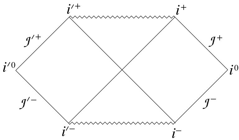
Figure 37. The Penrose diagram for the Schwarzschild black hole. The right quadrant describes the asympotically flat region external to the black hole. The upper quadrant is the black hole and the lower quadrant a white hole, each with spacelike singularities shown as jagged lines. The left quadrant is another asymptotically flat region spacetime.

The Penrose diagram allows us to give a more rigorous definition of a black hole. Here we’ll eschew any pretense at rigour, but give a flavour of the definition. We restrict attention to asymptotically flat spacetimes, meaning that far away they look like Minkowski space. This means, in particular, the asymptotic region includes both two null infinities, ${\mathcal{I}}^{+}$ and ${\mathcal{I}}^{-}$ . (We will further require that the metric looks like Minkowski space near ${\mathcal{I}}^{\pm }$ although we’ll be sloppy about specifying what we mean by this.) The black hole region is then defined to be the set of points that cannot send a signal to ${\mathcal{I}}^{+}$ . The boundary of the black hole region is the future event horizon, ${\mathcal{H}}^{+}$ Equivalently, the future event horizon ${\mathcal{H}}^{+}$ is the boundary of the causal past of ${\mathcal{I}}^{+}$ .

In the Penrose diagram of Figure 37, the black hole region associated to ${\mathcal{I}}^{+}$ is the upper quadrant and the left quadrant. The black hole associated to ${\mathcal{I}}^{\prime +}$ is the upper quadrant and the right quadrant.

Importantly, to define a black hole you need to know the whole of the spacetime: you run lightrays backwards from ${\mathcal{I}}^{+}$ and the boundary of these light rays defines the event horizon. There is no definition of the black hole region that refers only to a spacelike slice Σ at some moment in (a suitably defined) time. This means that an observer can’t really know if they’re inside a black hole unless they know the entire future evolution of the spacetime.

Relatedly, we can also define the white hole region to be that part of spacetime that cannot receive signals from ${\mathcal{I}}^{-}$ . The boundary of the white hole region is the past event

horizon, ${\mathcal{H}}^{-}$

6.1.5 Forming a Black Hole: Weak Cosmic Censorship

The Kruskal spacetime that we have discussed so far is unphysical in a number of ways. In reality, black holes do not emerge from white holes! Instead, they are formed by collapsing stars. The causal structure of such realistic black holes looks rather different from the Penrose diagram of figure 37.

We could try to write down solutions corresponding to collapsing stars. In fact, this is not too difficult. However, our main interest here is to understand the causal structure of the spacetime and we can do this by patching together things that we already know.

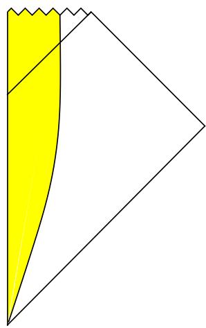
Things are conceptually most straightforward if we consider the unrealistic situation of the spherically symmetric collapse of a shell of matter. Inside the shell, spacetime is flat. Outside the shell, spacetime is described by the Schwarzschild geometry (6.1). Birkhoff’s theorem tells us that this latter statement remains true even for timedependent collapsing shells. If we further make the (again, unrealistic) assumption that the shell is travelling at the speed of light, then we can glue together the Penrose diagrams for Minkowski spacetime and the black hole spacetime, as shown in Figure 38. This gives the Penrose diagram for a collapsing black hole.

Although we made a number of assumptions in the above paragraph, the Penrose diagram that we derived also describes the spherical collapse of realistic stars. In this case, the surface of the star follows a timelike trajectory, as shown in the figure to the right. The unphysical parts of the Kruskal diagram have now disappeared: there is no white hole and no mirror universe.

Cosmic Censorship

One important feature of the black hole remains: the singularity is shrouded behind the horizon. This means that the effects of the singularity cannot be felt by an asymptotic observer. We can ask: is this always the case? Or could we end up with a singularity which is

not hidden by a horizon. Such singularities are called naked singularities

Naked singularities are commonplace in solutions to Einstein’s equations. The white hole of the full Kruskal spacetime provides one example; the Big Bang singularity provides another. Yet another is provided by the Schwarzschild metric. This solves the Einstein equations for all $M.$ , but is only physical for $M\ge 0$ . With $M<0$ , we can write the Schwarzschild metric as

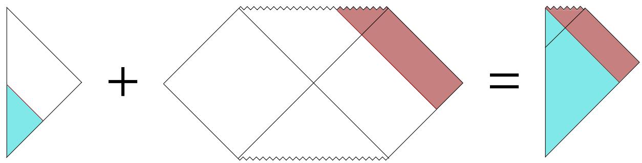
Figure 38. Joining two Penrose diagrams

$$d{s}^2=-\left(1+\frac{2G|M|}{r}\right)d{t}^2+{\left(1+\frac{2G|M|}{r}\right)}^{-1}d{r}^2+r^2(d{\theta }^2+{\sin }^2\theta d{\varphi }^2)$$

Now there is no coordinate singularity at $r=2G|M|$ and, correspondingly, no horizon. We can construct the Penrose diagram for this spacetime in the same way that we did for Minkowski space, now using null coordinates $u=t-r$ and $v=t+r$ . The final result is exactly the same as Minkowski space, with one difference: there is a curvature singularity at $r=0$ . The Penrose diagram is shown in the left-hand figure above. The singularity of the $M:<0$ black hole is not shielded behind a horizon. It is a naked singularity whose effects can be observed from ${\mathcal{I}}^{+}$

Despite the ubiquity of naked singularities in solutions to the Einstein equations, there is a general belief that they are unphysical. (The Big Bang singularity is an important exception to this and we will comment further on this case below.) A deep conjecture in general relativity, known as weak cosmic censorship, says that naked singularities cannot form. To phrase the cosmic censorship conjectures precisely, we would need to discuss the initial value problem in general relativity. The initial conditions are specified on a spatial hypersurface and are subsequently evolved through the equations of motion. The weak cosmic censorship conjecture states the following

The Weak Cosmic Censorship Conjecture: Given matter which obeys the dominant energy condition (described in Section 4.5.7), generic, smooth initial conditions for both the metric and matter fields in an asymptotically flat spacetime will not evolve to form naked singularities.

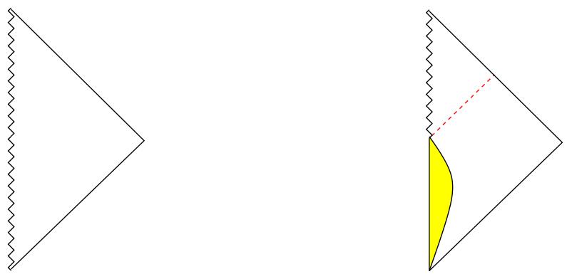
Figure 39. On the left: the Penrose diagram for a negative mass black hole. On the right: this kind of collapsing star scenario is forbidden by weak cosmic censorship.

There are a whole bunch of caveats in this statement. Each of them is important. It turns out that it is possible to construct finely tuned initial conditions (of measure zero in the space of all initial conditions) that result in naked singularities; hence the need for the word “generic”. It turns out that it is also possible to violate weak cosmic censorship in asymptotically AdS spacetimes. Finally, the naked singularity of the $M<0$ black hole gives some intuition for why we need the energy of the matter fields to obey some positivity condition.

If weak cosmic censorship is true, then it rules out dynamical evolution such as that shown in right hand figure. In fact, this diagram is somewhat misleading. Once the singularity forms, we can no longer evolve the fields beyond the light-ray shown as a dotted red line in the figure. This means that, strictly speaking, the dynamical evolution stops at the red line and can’t be extended beyond. A more precise statement of the weak cosmic censorship conjecture hinges on this idea and, in particular, the statement that $I^{+}$ doesn’t just come to an abrupt end.

There is no proof of weak cosmic censorship: indeed, it is arguably the biggest open question in mathematical relativity. Nonetheless, a wealth of numerical and circumstantial evidence supports the claim.

What should we make of cosmic censorship? At a practical level, it is a boon for those who work on numerical relativity, since it means that the simulations can proceed without worrying about how to cope with singularities. But for the rest of us, cosmic censorship is rather disappointing. This is because singularities – or, more generally, regions of high curvature – are where we expect quantum gravity effects to become important. Cosmic censorship means that it is unlikely we will have observational access to such behaviour. It is both striking and surprising that classical gravity finds a way to protect us from the ravages of quantum gravity.

There is one naked singularity that does appear to be physical: this is the Big Bang singularity. Since this lives in the far past, it certainly doesn’t violate the cosmic censorship conjecture. It’s tempting to think that we may ultimately be able to see the effects of quantum gravity here. Sadly, this hope too seems to be quashed, with inflation washing away the details of the very early universe. Quantum gravity is, it seems, a difficult observational science.

6.1.6 Black Holes in (Anti) de Sitter

Throughout this section we have focussed on black holes in asymptotically Minkowski spacetime. It is not hard to find solutions corresponding to Schwarzschild black holes in de Sitter and anti-de Sitter spacetimes, solving the Einstein equations

$$R_{\mu \nu }=\Lambda g_{\mu \nu }$$

We have already done the hard work. We take the ansatz

$$d{s}^2=-f(r{)}^{2}d{t}^2+f(r{)}^{-2}d{r}^2+r^2(d{\theta }^2+{\sin }^2\theta d{\varphi }^2)$$

We saw in Section 4.2 that this obeys the Einstein equations provided that

$$f^{\prime \prime }+\frac{2f^{\prime }}{r}+\frac{f^{\prime 2}}{f}=-\frac{\Lambda }{f}\text{ and }1-2f{f}^{\prime }r-f^2=\Lambda r^2$$

These equations have the solution

$$f^2=1-\frac{2GM}{r}\mp \frac{r^2}{R^2}$$

with $R^2=3/|\Lambda |$ . Here the minus sign solves the equation with $\Lambda >0$ and the plus sign with $\Lambda <0$ They correspond to black holes in de Sitter and anti-de Sitter spacetimes respectively. To see that this is the right interpretation, consider the metric with $2MG\ll R^2$ , so that the Schwarzschild radius is much less than the curvature of spacetime. Then, for $r\ll R,$ the metric looks like that of a Schwarzschild black hole in flat space. We will not have anything more to say about these solutions in these lectures.

来源与版本

正文：英文 · OCR 机器稿 · 待校对

核对状态：OCR 机器稿 · 待校对

原书 PDF

来源版本：michaelmas-2019-source-20260923

来源 PDF SHA-256：3ba65dc61f22a69c7d5fdf3e8e1f641efbfa6cf49a44b3dcb0fd5367ba9fcf1c

OCR 来源 SHA-256：5bbc97c50eaf0b03554f3ef1174075158c1598ac18f79242ddcda9dd2f12f618

OCR 产物 SHA-256：3e4949f8da98d66b99cd8ba79ae6e1435fe7a31371b630c93787a4862a52ae91